Adding the Topology ToolKit (TTK) to ParaView

Topological Data Analysis is coming to ParaView!

The Topology ToolKit (TTK) is now available in the ParaView nightly and in the latest release (v5.10), as well as in the ParaView Superbuild. TTK is a collection of filters specific to Topological Data Analysis (Contour tree, Morse-Smale Complex, Topological Simplification, …). You can load this plugin using the Tools > Manage Plugins… interface:

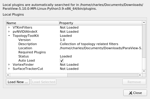
If you unfold the TopologyToolKit entry, you can click on Auto Load to make it directly accessible once you restart ParaView.

1. How to

When using TTK, the first step is to check that our data is a valid simplicial complex (we will define this notion formally later). In practice, if we are working with regular grids there is nothing to do. If we are working with explicit meshes, we may need to use Tetrahedralize and Clean to Grid to ensure the mesh only contains valid cells.

Let’s try our first pipeline. Taken from the TTK Examples website: the dragon.

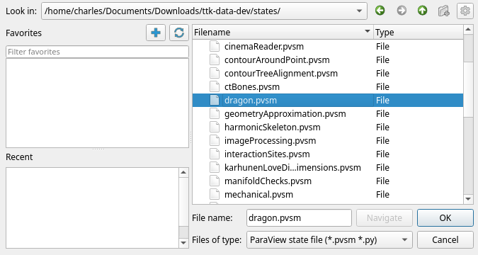
TTK examples rely on the ttk-data repository. You can download the corresponding archive here. Once you have downloaded / extracted the ttk-data, let’s start ParaView. Please ensure the TopologyToolKit plugin is loaded as seen Figure 1. Using the File > Load State menu, we select the dragon.pvsm entry inside ttk-data/states:

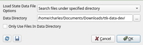
In the next menu, ParaView asks about State Data Files Options. As we want to use those in the archive, we select Search files under specified directory, and set the Data Directory to our ttk-data archive as shown in Figure 3.

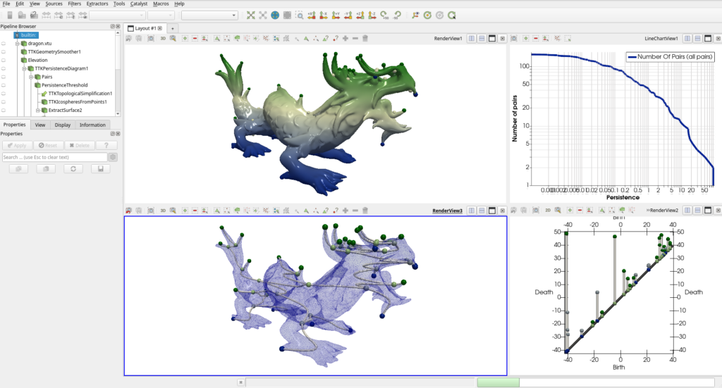
You should obtain the same result as shown in the example website, and Figure 4.

Some other great resources to understand TTK include tutorials and a beautiful gallery. All images in the gallery can be reproduced using the same method as we just used for the dragon state file. For typical pipeline panorama, please checkout the new TTK example website, which includes for each pipeline: a screenshot, a short pipeline description, the command line to reproduce the screenshot, a short python script to reproduce the pipeline, and pointers to the developer documentation.

2. Some notions of computational topology

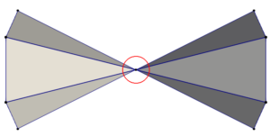
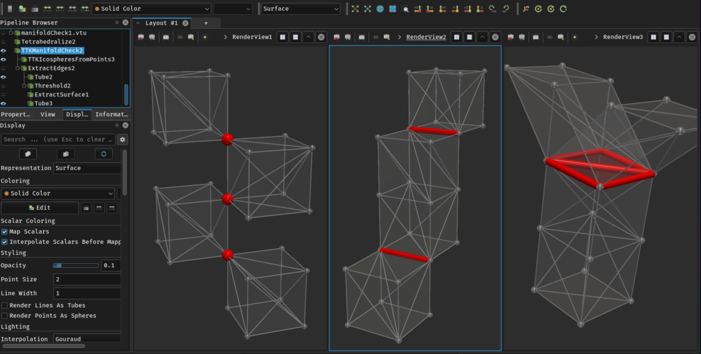
TTK assumes your input data is a simplicial complex. Intuitively simplicial complices are meshes only composed by vertices, edges, triangles and tetrahedrons (for dimension 3 or less). Additionally, for now, TTK requires manifold input meshes. In a manifold the neighborhood of each point is always composed of a single connected component. Figure 5 presents an example of an invalid mesh:

Acquisitions or simulations typically produce large data sets (defined as scalar fields on meshes), which are difficult to analyze and visualize and for which advanced tools are needed, to extract the core, structural information. That is the purpose of Topological Data Analysis (TDA). This is done through the use of topological abstraction, that can be seen as datasets maps. Depending on the kind of feature and relationship we study, we may want to choose the right map, the right abstraction. For example:

If we want to look at the regions of influence of extrema, we may use a level-set based topological abstraction like the Reeb Graph / Contour Tree, as shown in Figure 6:

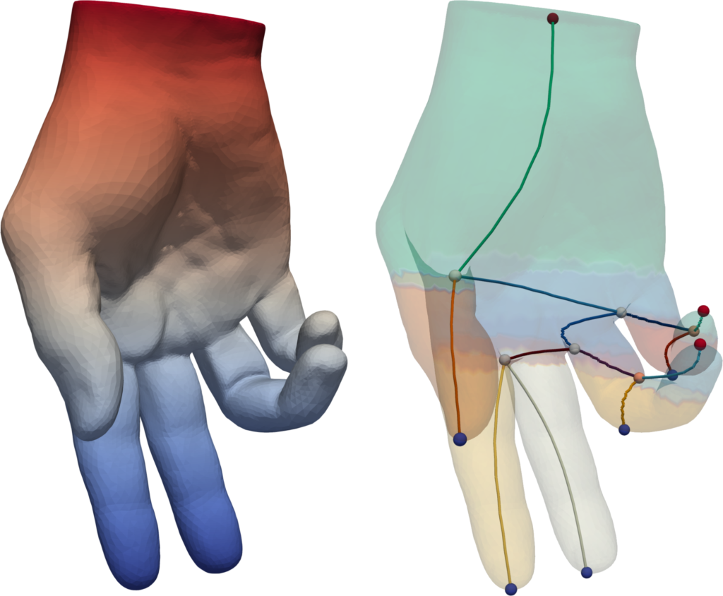
In this example, we can see how each minima / maxima at the end of the fingers correspond to a leaf arc and its corresponding region. These regions merge together at internal nodes in the tree. Due to its hierarchical nature, this tree also embeds a relationship between features, which can be used, for example, for noise removal.

TTK contains other kinds of topological abstractions that may be used when studying:

• the slope/gradient (Morse-Smale Complex)
• feature robustness and noise amount (Persistence Diagram / Chart)
• the temporal evolution of features (Planar Graph Layout)
• the relationship between various scalar fields (Continuous scatter-plot)

The toolkit also comes with filters to work with these abstractions. It is for example possible to hierarchically simplify the scalar field using the relationship emphasized in Figure 6. For a more complete introduction to Topological Data Analysis, you can find this IEEE Vis 2020 Tutorial: https://youtu.be/l5CjWChCVbM (Introduction starts at 00:06:55).

3. A segmentation example

Now, let’s use what we have seen in section 1 and 2 in an analysis pipeline. The goal here will be to extract regions corresponding to the bones along with the corresponding segmentation, on a human foot scan.

This corresponds to the ctBones.pvsm example, which we can load with the same method used in Section 1, to obtain the result shown in Figure 7:

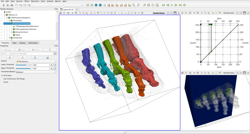
This state file reads the dataset ctBones.vti, containing a human foot scan with the density of matter represented as point scalars. Points with the highest density correspond to bones, and the lowest density is the air around the foot. Due to small fluctuations, especially in the air, this dataset is noisy. In the first part of the pipeline, we use a topological abstraction named the persistence diagram to extract the data set features. On this diagram, each bar corresponds to one feature and the persistence (the height) of the bar is a measure of the robustness of this feature. With a threshold on the persistence, we filter this diagram to only keep the most prominent features (see the Properties panel on the left of Figure 7). Then, the filtered diagram is used to configure a topological simplification of the initial domain, resulting in a new version where the noise has been removed.

With the TTK FTM Tree filter, we compute the contour tree along with the corresponding segmentation (cf. Section 2). Finally, we use this segmentation to extract areas attached to maxima. You can find a more detailed version of the pipeline in the tutorial that was given at IEEE VIS 2020: https://youtu.be/l5CjWChCVbM (time-code 01:38:45) and in the example website.

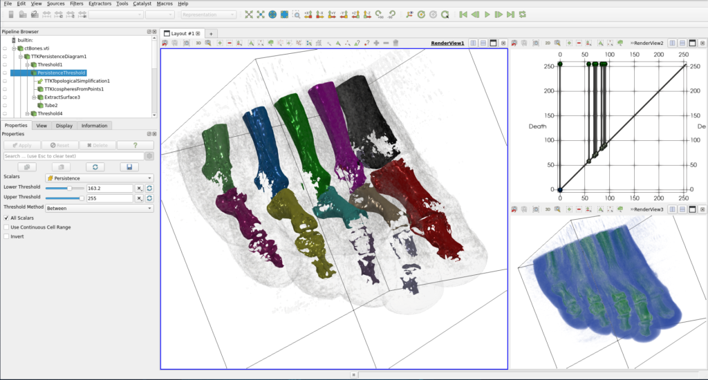
If you want to change the coarseness of the extracted feature, you can play with the “Lower Threshold” of the Persistence Threshold filter in the Pipeline. Figure 8 presents another example where we can distinguish phalanges.

In the gallery, we can find other pipelines that can be used to track vortices in a von Kármán simulation, extract region of influence in an atomic dataset, to do clustering using persistence or density gradient, to reconstruct a geometry from a cinema database, …

4. TTK on your own data

When using TTK, as explained in Section 2, you need to check that your data forms a manifold simplicial complex. For the simplicial complex part, the Thetrahedralize and Clean to Grid filters should be enough to ensure you only have valid cells. For the moment, you also need to check if your data is manifold. This can be done using the TTK Manifold checker filter. Its use is highlighted in this example, and illustrated in Figure 9.

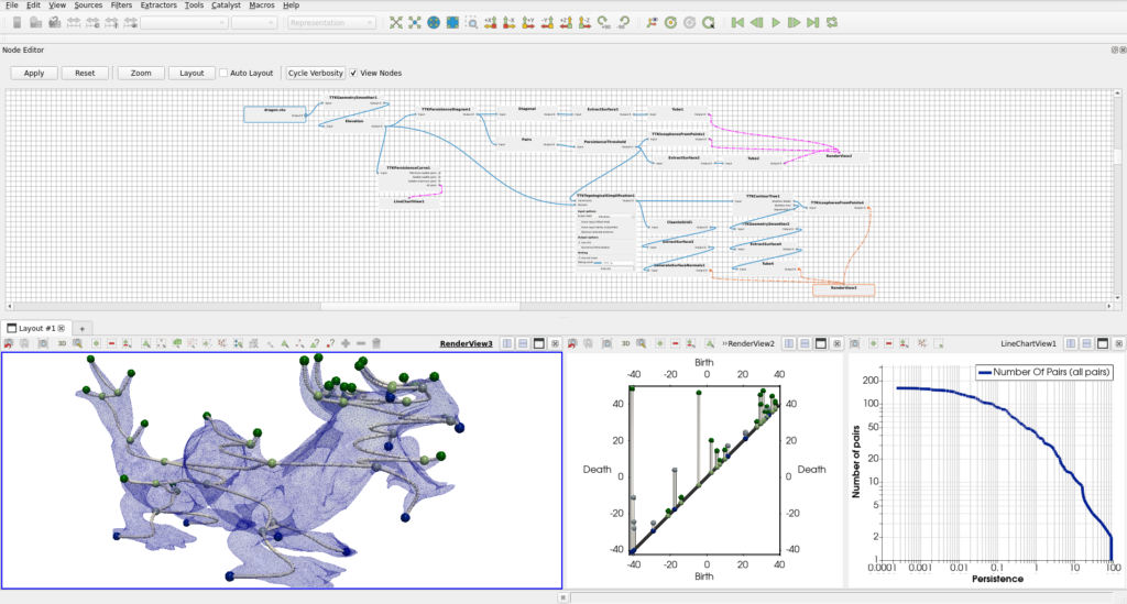
As a side note, using TTK often involves large pipelines. We may have a look at the recently added Node editor to replace / complement the original Pipeline browser. This Node editor is only available in the nightly version of ParaView and needs to be enabled using the Manage Plugins… menu that we saw earlier. A future blog-post will present this tool and how to use it, Figure 10 presents the dragon analysis shown Section 1 along with the Node editor:

5. TTK For developers

If you are a developer, the TTK website has a lot of resources to offer on:

• How to install TTK from sources
• How to use TTK in Python
• How to use TTK in VTK/C++
• How to use TTK in pure C++
• How to extend TTK

TTK’s architecture is based on modules, so it can be easily extended. Contributors may add their own algorithm and wrap them in VTK / ParaView with a minimal effort.Here again, we have a step-by-step tutorial (see Video 1).

These modules benefit from the TTK Triangulation data model which enables for fast traversal and efficient neighborhood requests on the input domain.

Last but not least, we have a welcoming community. If you have any questions or remarks, join us on https://groups.google.com/g/ttk-users. The github is also a good place if you have troubles of suggestion regarding TTK.

Acknowledgements

This work was partially supported by the European Commission grant H2020-FETHPC-2017 “VESTEC” (ref. 800904).