Tracking droplets in multiphase flow simulations using ParaView, MegaMol and some custom bits
This post is an invited guest blog by: Matthias Ibach, Alexander Straub and Moritz Heinemann researchers at the University of Stuttgart.
Multiphase flow simulations: what, why and how?
“Any object, totally or partially immersed in a fluid or liquid, is buoyed up by a force
Archimedes’ Principle
equal to the weight of the fluid displaced by the object.”
Archimedes of Syracuse, who postulated the laws of buoyancy more than 2,000 years ago (known as Archimedes’ principle), created one of the very first works of humankind related to flows that involved multiple phases. Even nowadays, such multiphase flows – which describe a flow of materials with two or more distinct thermodynamic phases – are still an important research topic. This is hardly surprising as multiphase flows are ubiquitous in our everyday life. We encounter them, for example, as sprays for body care, waves at the beach, or even at the dripping bottle edge of red wine.
In many engineering problems, two or more phases interact, which are often a liquid and a gaseous phase. Some current investigations, technologies, and applications of multiphase systems encompass biofuel sprays in gas turbine engines or concepts of injecting exhaust heat-generated steam into the combustion chamber of an aero engine, both to reduce pollutant emissions and increase efficiency.
Natural Multiphase Flows
There are many more examples, where we come across multiphase flows on a daily basis.
Some examples in nature are comprised of raindrops, dew, fog or haze relevant for accurate modeling of weather forecast in meteorology [i], groundwater flow in soil as porous medium [ii] or even the role of ocean sprays on the formation of tropical cyclones or global climate [iii].
[i] https://doi.org/10.1175/2009JAS3174.1; https://doi.org/10.1175/2009JAS3175.1
[ii] https://doi.org/10.1016/j.advwatres.2012.07.003
[iii] https://doi.org/10.1017/jfm.2020.314
Industrial Multiphase Flows
Other fields of relevance in industrial use of multiphase flows cover spray coating methods for solar cell fabrication [iv] or spray cooling of microchips, the effective operation of medical inhalators [v], the production of capsules in pharmaceutical applications [vi], mitigation of pesticide spray drift [vii] or fertilizer in agriculture, 3D ink-jet printing [viii], or heat supply in form of regenerative and environmentally friendly geothermal energy through phase change processes within corrugated tubes [ix].
[iv] https://doi.org/10.1016/j.mssp.2015.05.019
[v] https://doi.org/10.1016/j.ejpb.2021.05.021
[vi] https://arxiv.org/abs/2212.09727v1; https://doi.org/10.1016/j.colsurfa.2009.12.011
[vii] https://doi.org/10.1016/j.cropro.2012.10.020
[viii] https://doi.org/10.1063/1.5087206
[ix] https://doi.org/10.1007/s00231-017-2014-7; https://doi.org/10.1016/j.jppr.2017.05.002
In many of these cases, the key to achieving the desired outcome lies in the precise control of the system and a deep understanding of the physics involved. With increasing computational power, highly temporally and spatially resolved computational fluid dynamics (CFD) simulations can be employed to shed light on essential physics on small scales. State-of-the-art in this regard are direct numerical simulations (DNS) with interface tracking schemes.
However, due to the dynamics and complexity of such multiphase flows—phenomena such as collision, deformation, adhesion, breakup, or strong topological changes with detachment of droplets and ligaments can occur—the analysis of the resulting data is highly challenging due to their spatio-temporal nature. Data sizes can quickly reach terabytes, burying important interrelations of quantities of interest in the degrees of complexity of the acquired data, not directly reachable for engineering investigation anymore. This is where ParaView’s customizability and modularity come in handy to tailor post-processing pipelines fitting the needs of such specific multiphase flow applications and problems.
From simulation…
For over 25 years, the in-house code Free Surface 3D (FS3D) [1] has been developed at the Institute of Aerospace Thermodynamics (ITLR) to investigate such multiphase flows with direct numerical simulations.
The code is based on the volume of fluid (VOF) method [6] and solves the Navier-Stokes equations for incompressible flows on finite volumes (FV) on a Cartesian grid arrangement. Additionally, the energy equation can be solved, including the option of phase change processes, such as evaporation, sublimation, or freezing. Surface tension forces can be calculated in different ways: By the conservative continuous surface stress (CSS) model or the balanced force approach (bCSF). FS3D employs a staggered grid, velocities are saved on cell faces while scalar values are stored in the cell centers (marker-and-cell (MAC) method). To determine the velocities, both mass and momentum equations are solved simultaneously. Convective terms are calculated with a second order upwind scheme while diffusive fluxes are determined using central differences, also of second order. The fluxes are obtained through Godunov schemes. A total variation diminishing (TVD) limiter restricts the spatial derivatives to avoid the occurrence of new velocity maxima. For the advection of scalars, three one-dimensional non-conservative transport equations are solved successively according to the Strang splitting method. A novel implementation consisting of an improved advection scheme following the formulation of Weymouth and Yue was added to the code framework, guaranteeing full mass conservation. As a result of volume conservation of an incompressible flow, a Poisson equation has to be solved for the pressure. Here, a multigrid solver is used. A red-black Gauss-Seidel algorithm has been implemented as a smoother and the whole solver can be run either as a V-, W- or F-cycle.
The simulations with FS3D focus mainly on the mass, momentum, and heat transfer across interfaces. Due to the investigated processes happening on very small scales and because of the absence of turbulence models, DNS inherently requires a very high resolution of the computational domain. In this context, the use of modern high-performance computers is indispensable. The existing code is parallelized using OpenMP and MPI (hybrid parallelization) and is suitable for the efficient calculation of complex flow and thermodynamic phenomena. It is adapted to run efficiently on the HPE Apollo supercomputer “Hawk” at the High-Performance Computing Center Stuttgart (HLRS).
We investigated many relevant fundamental processes spanning areas from multiple droplets impacting onto thin films or structured surfaces, droplet-droplet interactions and clustering (“droplet grouping”), the injection of water droplets into a compressor cascade of gas turbines to reproduce the interaction between the blades and the liquid phase, and we are even performing sophisticated numerical simulations of primary breakups of liquid jets with non-Newtonian material properties with approximately 2.5 billion computational cells [2,3,4,5].
The additional presence of a (freely moving) interface between the different phases makes numerical modeling, analysis, and visualization much more complex than in single-phase flows. To identify each phase and, accordingly, the phase boundary, the Volume-of-Fluid (VOF) method [6] is employed in FS3D. It is a volume tracking method where an additional volume fraction f is introduced corresponding to the volume of the disperse phase, i.e., the non-continuous phase, in each cell. Thus, it can take values between 0 and 1. For the computation of the VOF fluxes, FS3D uses a piecewise linear interface calculation (PLIC) algorithm, which reconstructs the interface with planar segments. These segments are oriented along the gradient of the volume fraction in the respective cells, separating the continuous and the dispersed phase and keeping the interface sharp.
… to first visual overview
The first step is to load the data to provide the domain experts with visualizations of their simulations. These data are stored in the proprietary FS3D data file format or as HDF5. For both, we developed readers to provide specific capabilities to read the input scalar and vector fields. The most important of these are the VOF and velocity fields. Furthermore, the data can include interface forces, pressure, interface gradients, curvatures, and other simulated quantities.
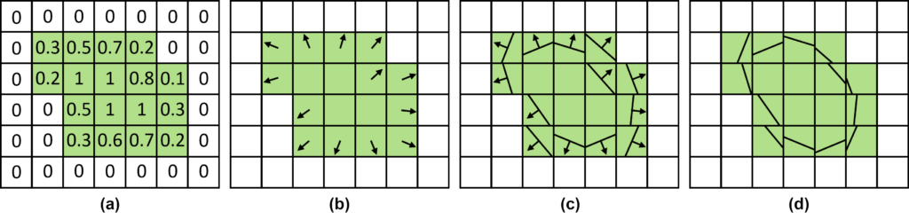
ParaView already offers filters for interface reconstruction, such as Marching Cubes (contour filter), which we can use on the now-loaded VOF data to visualize the shape of the droplets. These data consist of a scalar value per cell in a Cartesian grid. Thus, the droplet interface can be directly extracted from the VOF field by choosing an isovalue between zero and one. While the isosurface provides a continuous surface representation, it does not maintain the property of enclosing the correct volume as indicated by the VOF values. To get a representation that retains the correct volume, albeit with the downside of discontinuity between neighboring cells, we implemented PLIC as a ParaView filter in our two-phase flow (TPF) framework (cf. section on implementation). Thus, we provide the simulation researchers with a simulation-oriented visualization [7]. As input, it only requires the VOF field, calculates the VOF gradient, and applies a binary search to fit the resulting PLIC plane to approximate the enclosed volume of the VOF field. This process is depicted in Figure 1.
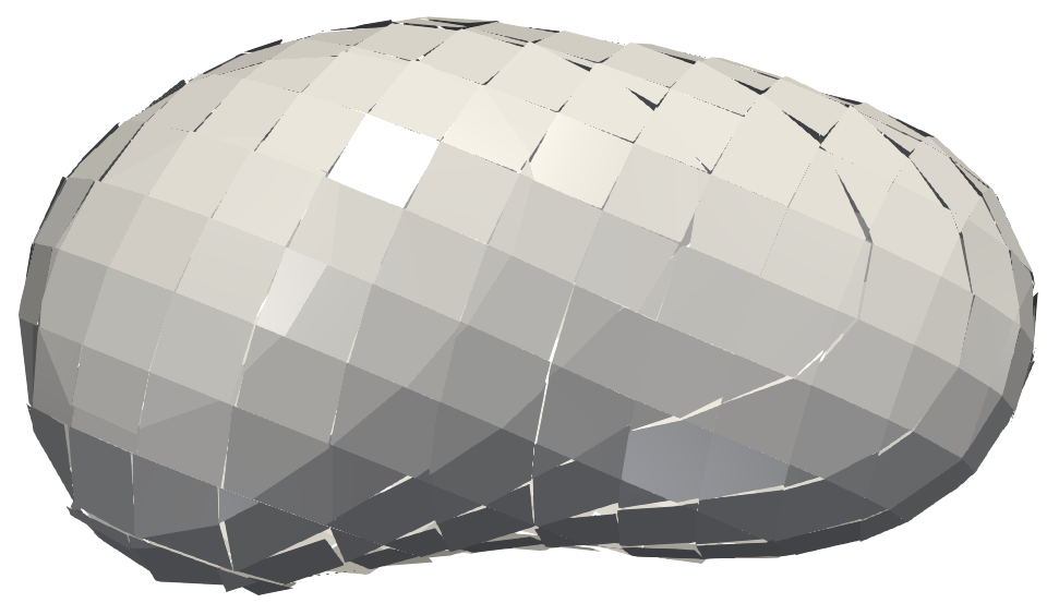
As a result, PLIC is a basic but domain-specific approach whose output consists of a single polygon per cell. An example showing the reconstructed interface of a droplet is shown in Figure 2.
Until now, we have always assumed to have only two fluid phases, i.e., a liquid phase (e.g., water droplet) and a surrounding gas phase (e.g., air). However, there are applications with more than two phases. Multiple VOF fields are generated in such simulations, one for each fluid phase. Therefore, we also implemented a version of PLIC that can handle three-phase flows, i.e., simulation data with three different immiscible fluids or two fluids and a solid phase.
Scientific Visualization and ParaView
The processing pipeline is one of the basic concepts in visualization. It describes in a general way how data is processed and transformed on its way to our screen. The ParaView pipeline takes a similar approach, where data is loaded or created by a source, transformed and mapped to visual primitives by filters, and finally rendered using a representation. The similarity of the concept becomes apparent when looking at the diagram in Figure 3. Here, you can see the steps of the visualization pipeline in black and the stages from ParaView in green. As an example, we take again the reconstruction of the PLIC surface. Using a source, VOF data are loaded from files. They are then processed to add gradient information, mapped to a surface mesh, and rendered into a ParaView window.
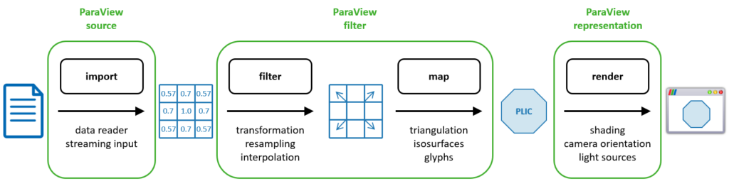
The apparent advantage of ParaView for visualization researchers is the large number of modules readily available at each stage in the visualization pipeline, and their interoperability. On the one hand, this allows us to quickly look at data using the already provided data sources, filters, and representations. Suppose our data require more specific algorithms for analysis. In that case, we can add custom data sources and filters using the Python or C++ API. On the other hand, our domain scientists can thus stay within their well-known ParaView environment and simply add the visualization modules we provide.
Visualizing Flow within Droplets
Analyzing flow simulations, we are often interested in how the simulated liquid behaves over time. For visualizing the flow, we can use the concept of massless particles contained in droplets. Tracing these particles in our vector field results in curved lines that reflect their paths. We call such lines streamlines for static (constant-time) vector fields \(\mathbf{u}(\mathbf{x})\):
\(\displaystyle\frac{\partial \mathbf{x} (t)}{\partial t} = \mathbf{u}(\mathbf{x}(t)), \quad \mathbf{x}(0) = \mathbf{x}^{0},\)
and pathlines for dynamic (time-dependent) vector fields \(\mathbf{u}(\mathbf{x}, t)\):
\(\displaystyle\frac{\partial \mathbf{x} (t)}{\partial t} = \mathbf{u}(\mathbf{x}(t), t), \quad \mathbf{x}(0) = \mathbf{x}^{0}.\)
These equations state that the time-derivative of the position (left-hand side), i.e., the tangent of the resulting stream- or pathline, equals the velocity in the vector field (right-hand side). This means that the stream- or pathline is always parallel to the vector field. Position \(\mathbf{x}\) at time 0 is the starting point at which a line is seeded.
ParaView already implements the computation of stream- and pathlines in the Stream Tracer filter. You can see an example in Figure 4(a), (c) for the whole domain, and (b), (d) restricted to flow inside the individual droplet.
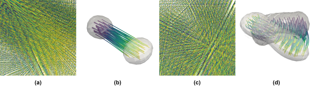
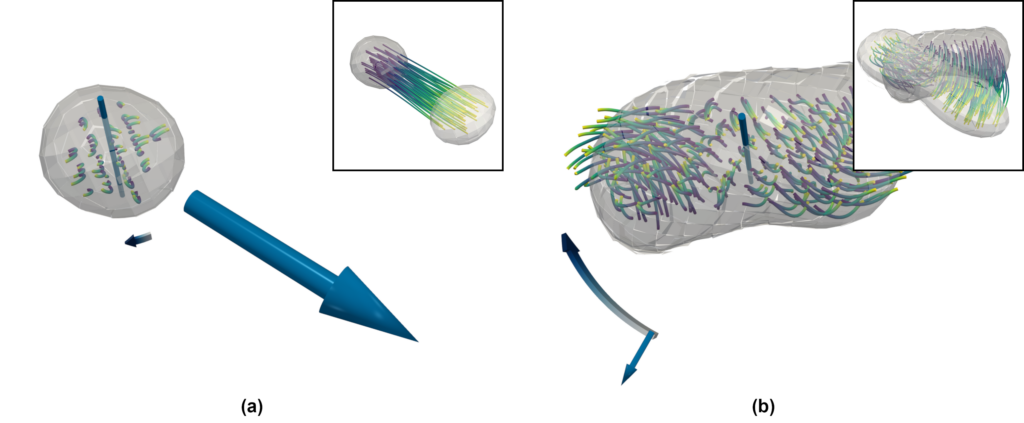
Note that in Figure 4(b) and (d), the visualizations are dominated by strong translation and rotation, respectively. Thus, it is hard to observe the local details of the flow. Therefore, we want to go one step further and look at the droplets locally [8]. This means that for now, we want our visualization to ignore the movement of the droplet itself. For this, imagine that every droplet is recorded by a different camera moving with the same velocity as the droplet. If the droplet itself is spinning, then the camera spins around the droplet as well. This idea allows us to visualize the flow as if the droplets were stationary. For this, we implemented ParaView modules at the visualization pipeline’s filter stage.
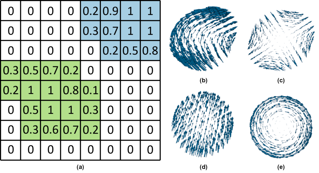
As a first step, we need to create a filter to identify droplets in our data. We do this directly in the VOF field by looking at all the cells that contain the liquid phase, i.e., cells with VOF value \(f \gt 0\). A droplet then consists of all these cells not separated by empty cells, as shown in Figure 5(a). The same filter also computes for all droplets their respective translational and rotational velocity from the input vector field. In our above analogy of a camera attached to a droplet, by moving the camera with the droplet, we get the droplet-local velocity field in the camera’s frame of reference as
\(\mathbf{u}^{local} = \mathbf{u}^{orig} – \mathbf{u}^{trans} – \mathbf{u}^{rot},\)
where orig denotes the original vector field, trans the translational part, and rot the rotation.
Droplet translation
The translational velocity of a droplet is defined as
\(\mathbf{u}^{trans} = \displaystyle\frac{\sum_{i}\rho_{i}V_i \mathbf{u}_{i}}{\sum_{i} \rho_i V_{i}},\)
where i denotes the cell index in our input grid pertaining to a specific droplet. Here, we can directly substitute the product of the density and the volume of the cell with our VOF value \(f\) to get
\(\mathbf{u}^{trans} = \displaystyle\frac{\sum_{i}f_i \mathbf{u}_{i}}{\sum_{i} f_{i}},\)
which now only depends on the values provided in our input grid. Note that we get one translational velocity per droplet. This means that the translational velocity is the same for all cells of the droplet.
Droplet rotation
Contrary to translation, the rotational velocity differs for all droplet cells. The angular velocity, however, is defined for the whole droplet as
\(\omega = I^{-1} L,\)
with inertia tensor \(I\) and angular momentum \(L\). Finally, the rotational velocity at the cell center \(\mathbf{r}\) of the droplet is defined as
\(\mathbf{u}_ {i}^{rot} = \omega \times \mathbf{r}_{i}´\)
where \(r_{i}’\) is the cell center’s position relative to the droplet’s center of mass
\(\mathbf{r}_{c} = \displaystyle\frac{\sum_{i}f_{i}\mathbf{r}_{i}}{\sum_{i}f_{i}}\)
For streamlines, we can now apply the Stream Tracer on the droplet-local vector field directly, which thus solves
\(\displaystyle\frac{\partial \mathbf{x}(t)}{\partial t} = \mathbf{u}^{local}(\mathbf{x}(t)), \quad \mathbf{x}(0) = \mathbf{x}^{0}.\)
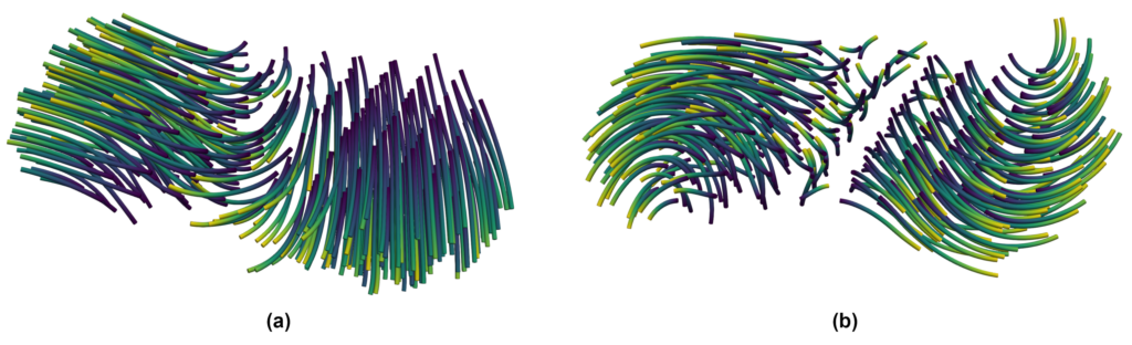
The result of this computation can be seen in Figure 6 for an example droplet, showing (a) the original streamlines and (b) the droplet-local ones. While the original streamlines would indicate a rapid disintegration of the droplet, the droplet-local view shows strong rotation at both ends.
Pathlines, on the other hand, require a new filter for their computation. For this, we have to modify the equation slightly. This is necessary to find the correct positions \(\mathbf{x}(t)\) where our velocity is defined, while creating our droplet-local pathline:
\(\displaystyle\frac{\partial \mathbf{x}^{local}(t)}{\partial t} = T^{-1}_{rot}\mathbf{u}^{local}(\mathbf{x}(t), t), \quad \mathbf{x}(0) = \mathbf{x}^{local}(0) = \mathbf{x}^0 .\)
For the implementation, this means that we need to compute the original pathlines as well in order to find the sampling locations \(\mathbf{x}(t)\). Additionally, we must undo the droplet’s rotation \(T\) by applying its inverse to our local vector field. Figure 7 shows an animation of the pathline computation.
Similar to ParaView’s Stream Tracer, the output consists of polylines. For visualization, their use is somewhat limited, as their width is always only one pixel, and shading cannot be used effectively to discern depth within the images. Therefore, we usually apply tube glyphs to our stream- and pathlines and adjust the scene’s lighting by, e.g., adding more light sources. All of this is already provided in ParaView and can easily be set up within the GUI.
The result can be observed in Figure 8 that shows the pathlines for the same two droplets as earlier (cf. boxes). With the droplet-local view, we can now better observe the local flow behavior within a droplet. To also show the information that we removed from the velocity field (translation and rotation), we add glyphs to the visualization.
Employing Machine Learning and Coupling With ParaView
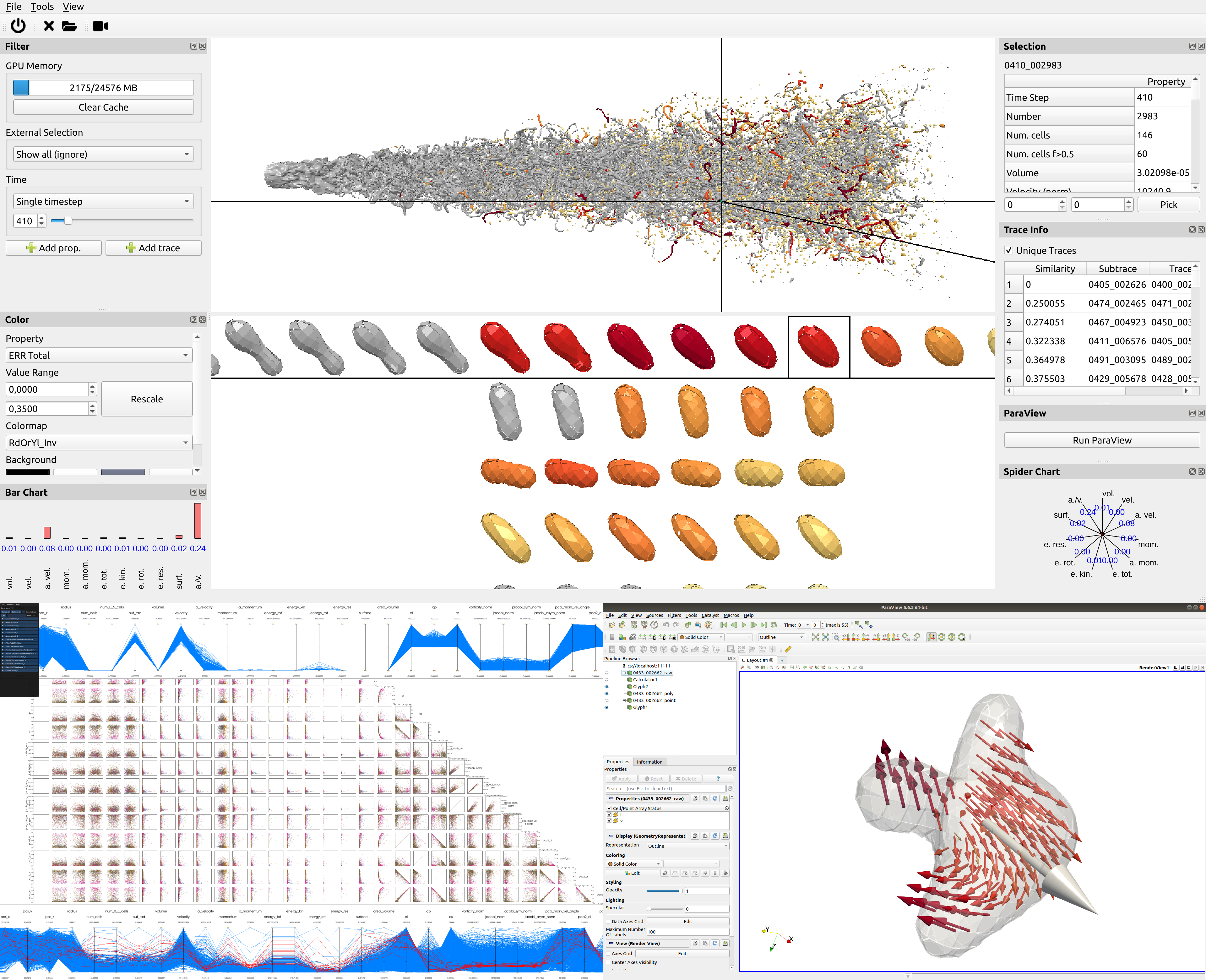
Analyzing droplet dynamics in sprays is relevant in many scientific and engineering fields. Unfortunately, the pure amount of thousands of droplets (see Figure 9) makes this a cumbersome task. We try to overcome this using a Machine Learning (ML) approach [9].
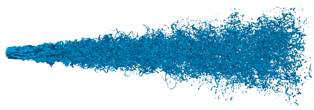
For this, droplets are first extracted, similar as in Figure 5(a), and traced over time. In addition, each droplet is reduced to a vector of its physical quantities, such as mass, velocity, angular velocity, different energy terms, etc. This is again similar to the above equations for droplet translation and rotation.
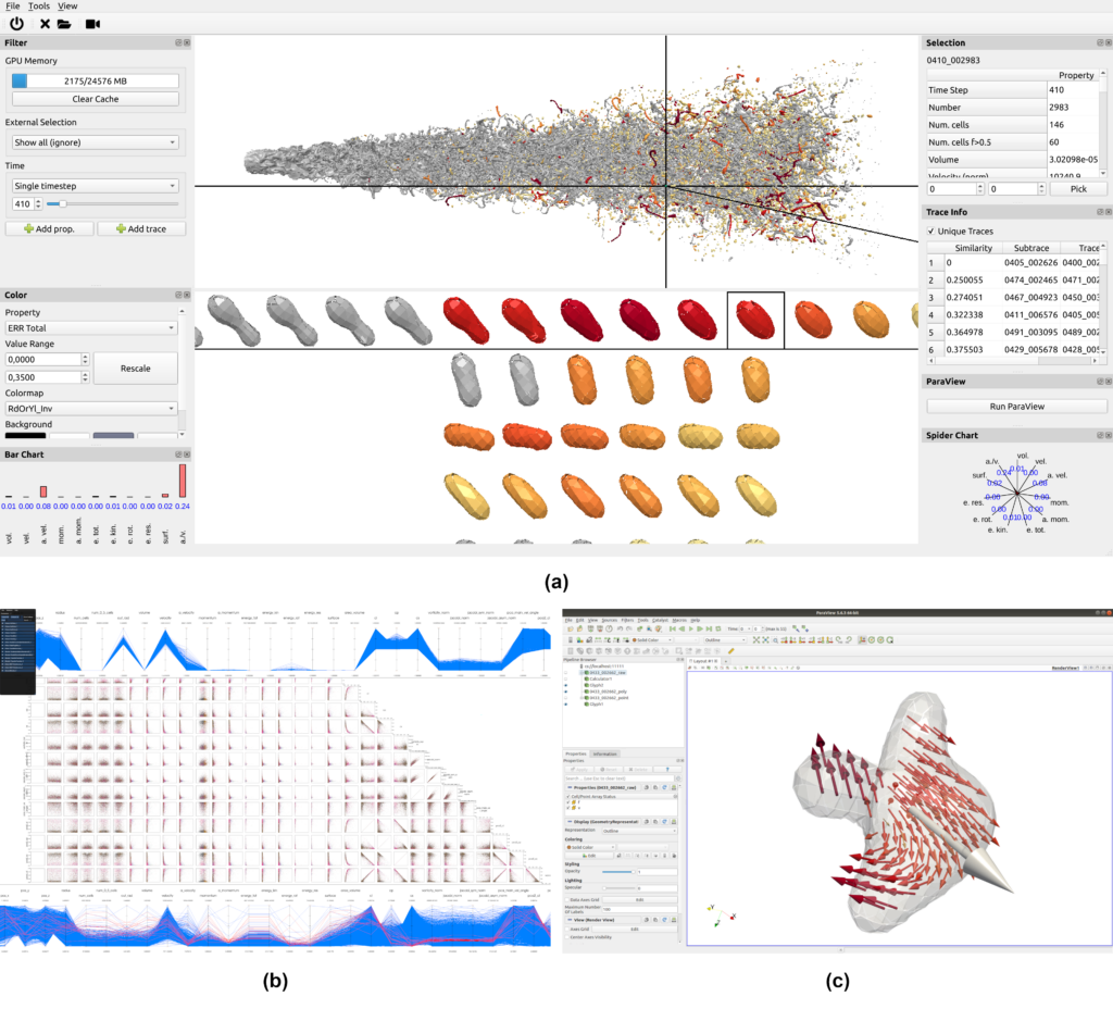
Next, we train a neural network as a regression model on the temporal development of these quantity vectors. We use temporal sub-samples of each droplet to predict the future development of the quantities and compare the predicted values to the actual physical quantities of that droplet at a later time step. Our hypothesis is that the error of this prediction correlates to how interesting a droplet is and if it merits further investigation.
To prove our hypothesis, we built a visual analytics tool from scratch for this specific scenario. In the beginning, we decided to develop a standalone application because we could directly build upon our ML pipeline. This was especially useful as the dataset was quite large and we could optimize the internal data structures to directly fit into GPU memory on a standard workstation computer.
While working on this tool, we reached a point where we wanted to investigate the flow field within single droplets and lacked the means to do so. In contrast, ParaView provides many filters suitable for that task. Of course, we could have just exported single droplets to load them independently in ParaView. However, that would have been a very tedious task for the user. To overcome this limitation, we found a way to directly integrate ParaView into our analysis tool. As ParaView supports connecting multiple clients to a single ParaView server, we utilize this setup in our application; we start a ParaView server and connect the default ParaView client to it, which can be used by the user as usual. In addition, in the background, our tool connects as a second client to the ParaView server, which allows to automate tasks. This means that the user can click on a droplet in our tool, and the data will be automatically loaded into ParaView with a default filter pipeline. Henceforth, the user can continue analyzing this single droplet with the full capabilities of ParaView.
External Resources
Implementation
The source code of our implementations is open source under the MIT license.
ParaView Plugins
We developed small ParaView modules for simple and recurrent tasks. For this, our modules provide functionality for converting grids of one type to another, manipulating input polylines, or providing sources for generating simple analytic geometry.
https://github.com/UniStuttgart-VISUS/ParaView-Plugins
TPF
At some point, we started to create our own small library TPF (two-phase flow) to develop modules that can be easily integrated into different frameworks. For ParaView, these modules are wrapped as filters with the appropriate VTK interface and module descriptors. Thus, our filters can be used in ParaView, with the prospect of integrating them easily into our in-house framework MegaMol, as well.
https://github.com/UniStuttgart-VISUS/tpf
Technical example
The following are the steps to remote control ParaView:
- Start the ParaView server:
./pvserver --multi-clients
- Start the ParaView client:
./paraview --url="cs://localhost:11111"
- Connect the Python client:
./pvpython /path/to/paraview-control.py
A toy example with data can be found here:
https://github.com/UniStuttgart-VISUS/paraview-multi-client-demo
Authors
Matthias Ibach studied Aerospace Engineering at the University of Stuttgart where he received his Bachelor’s and Master’s degrees. Since 2018, he has been a research associate at the Institute of Aerospace Thermodynamics (ITLR) at Uni Stuttgart where his field of research is the numerical investigation of multiphase flows, studying and analyzing basic phenomena such as droplet grouping, oscillation, and droplet-droplet and droplet-film interaction with the DNS in-house VOF code Free Surface 3D (FS3D).
Alexander Straub studied Computer Science at the University of Stuttgart, where he received his Bachelor’s and Master’s degrees. Since 2016, he has been a research associate at the Visualization Research Center (VISUS), where he works on the visualization of multiphase flow processes. These include visualizations for droplet interaction and flow in porous media.

Moritz Heinemann studied Simulation Technology at the University of Stuttgart, where he received his Bachelor’s and Master’s degrees. Since 2018, he has been a research associate at the Visualization Research Center (VISUS), where his work focuses on the visualization of droplet dynamic processes, but is also interested in rendering performance and power consumption.
References
[1] Kathrin Eisenschmidt, Moritz Ertl, Hassan Gomaa, Corine Kieffer-Roth, Christian Meister, Philipp Rauschenberger, Martin Reitzle, Kathrin Schlottke, Bernhard Weigand. Direct numerical simulations for multiphase flows: an overview of the multiphase code FS3D. Applied Mathematics and Computation, 272: 508–517, 2016. https://doi.org/10.1016/j.amc.2015.05.095
[2] Stephanie Fest-Santini, Jonas Steigerwald, Maurizio Santini, Gianpietro Elvio Cossali, Bernhard Weigand. Multiple drops impact onto a liquid film: Direct numerical simulation and experimental validation. Computers & Fluids, 214: 104761, 2021 https://doi.org/10.1016/j.compfluid.2020.104761
[3] Matthias Ibach, Visakh Vaikuntanathan, A. Arad, D. Katoshevski, J.B. Greenberg, Bernhard Weigand. Investigation of droplet grouping in monodisperse streams by direct numerical simulations. Physics of Fluids, 34(8): 083314, 2022. https://doi.org/10.1063/5.0097551
[4] Moritz Ertl, Bernhard Weigand. Analysis methods for direct numerical simulations of primary breakup of shear-thinning liquid jets. Atomization and Sprays, 27(4): 303–317, 2017. https://doi.org/10.1615/AtomizSpr.2017017448
[5] Adrian Schlottke, Matthias Ibach, Jonas Steigerwald, Bernhard Weigand. Direct numerical simulation of a disintegrating liquid rivulet at a trailing edge. High Performance Computing in Science and Engineering ’21, pp. 239–257, 2023. https://doi.org/10.1007/978-3-031-17937-2_14
[6] C.W. Hirt, B.D. Nichols. Volume of fluid (VOF) method for the dynamics of free boundaries. Journal of Computational Physics, 39(1): 201–225, 1981. https://doi.org/10.1016/0021-9991(81)90145-5
[7] Grzegorz K. Karch, Filip Sadlo, Christian Meister, Philipp Rauschenberger, Kathrin Eisenschmidt, Bernhard Weigand, and Thomas Ertl. Visualization of piecewise linear interface calculation. IEEE Pacific Visualization Symposium, PacificVis 2013, pp. 121–128, 2013. https://doi.org/10.1109/PacificVis.2013.6596136
[8] Alexander Straub, Sebastian Boblest, Grzegorz K. Karch, Filip Sadlo, and Thomas Ertl. Droplet-Local Line Integration for Multiphase Flow. 2022 IEEE Visualization and Visual Analytics (VIS), pp. 135–139, 2022. https://doi.org/10.1109/VIS54862.2022.00036
[9] Moritz Heinemann, Steffen Frey, Gleb Tkachev, Alexander Straub, Filip Sadlo, and Thomas Ertl. Visual Analysis of Droplet Dynamics in Large-Scale Multiphase Spray Simulations. Journal of Visualization, 24(5): 943–961, 2021. https://doi.org/10.1007/s12650-021-00750-6
Acknowledgments
Funded by Deutsche Forschungsgemeinschaft (DFG, German Research Foundation) as part of Germany’s Excellence Strategy in EXC 2075 “SimTech” (390740016), GRK 2160 “DROPIT” (270852890), Investigation of Droplet Motion and Grouping (409029509), SFB-TRR 75 (84292822), SFB-TRR 161 (251654672), SFB 1313 (327154368), and the High-Performance Computing Center Stuttgart (HLRS) (FS3D/11142).
What fantastic work this is! I am floored by the quality of this effort. I hope that you publish this work at one of the major vis conferences as there is much novelty in it. Thank you for sharing it.