Configurable and Parallel Task Graph in iMSTK

Introduction

iMSTK 3.0 introduced task graphs to allow flexibility in the configuration of the computational pipeline as well as to add scene-level task parallelization. Task graphs allow users to create computational blocks as nodes and to specify edges that determine the order of execution. Expressing computation using the task graph makes it easier to take advantage of scene-level task parallelism that is often not captured by loop-based parallelization.

Motivation

iMSTK currently supports simulation of rigid bodies, elastic objects, and fluids for potential use in interactive multi-modal surgical simulation. iMSTK’s dynamical model classes implement the mechanisms to evolve time-dependent physical quantities (e.g. positions, velocities, temperatures, stresses, or pressures) of objects. The user may choose to use different numerical approaches that model the underlying governing equations. iMSTK current supports position-based dynamics (PBD), smoothed particle hydrodynamics (SPH), finite elements, and rigid body dynamics dynamical models. These models vary widely in the number and type of steps (see Figure 1) and exist because they are better suited for different situations. Some models may be better for fractures, large deformations, while others are specifically used to enforce incompressibility and so forth. For this reason, one may employ multiple models during a surgical scenario. However, the specifying interaction between these disparate models can quickly become cumbersome without highly coupled code.

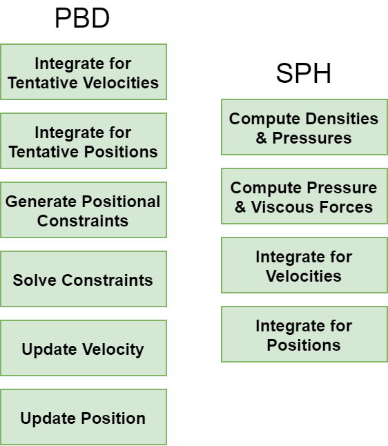
Figure 1: Simplified PBD and SPH dynamical models showing different sub-steps. Each model has many variations.

Configurability of the Computational Pipeline

Currently, iMSTK defines a set of stages for the physics pipeline with a fixed ordering. At a high level, first, the inter-object collisions are detected, then collision handlers are run, solvers are executed (which invokes dynamical models that advance the model in time) and finally the geometric mappers update the geometry. The heterogeneity of the dynamical models makes this fixed order limiting and hard to customize. For example, some dynamical models may want collision detection to be done after intermediate state updates. Some may even need to do different types of collisions in a single advance. There is really no telling what a user could come up with to advance a model in time. Task graphs remove the need for the iMSTK scene to enforce a fixed ordering thus allowing considerable flexibility in reconfiguring existing models or implementing a new model altogether.

Task-based Parallelization

iMSTK has been increasingly taking advantage of multi-processor CPUs as we further explore data, loop, and task-based parallelism. iMSTK has been using Thread Building Blocks (TBB) for loop-based parallelism. While this utilizes the CPU well, it is not optimal and largely depends on the composition of the scene and the hardware it is running on. The inter-object interactions specified as part of the scene often dictate whether the dynamical models of those objects can be updated in parallel. Prior to the task graph, scene-level interdependencies (or lack thereof) were not used to optimize parallel execution. Besides, it may be nearly impossible to express this via loop-based parallelism.

Task Graph

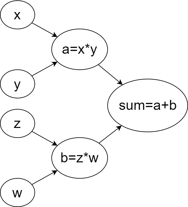
To address these concerns we introduced task graph, which is a directed graph of nodes where each node represents a computational task to be scheduled. This could be a simple algebraic expression in a computational graph (see Figure 2 for example) or it could be high-level computational steps of a dynamical model (shown in Figure 1) such as the integration of velocities or computation of densities in SPH.

iMSTK Task Graphs

iMSTK’s task graph is a directed acyclic graph with a single entry and a single exit also called source and sink respectively. It contains a set of task nodes and directed edges between them that define the flow of control between the task nodes. In the context of parallel computation, when a node splits, there may be an opportunity to run its successors in parallel. When nodes merge, threads need to synchronize.

Usage

Here is a code showing the usage of task graphs in iMSTK for the sample task graph shown in Figure 1.

//Inputs
const int x = 0, y = 2, z = 3, w = 5;
std::shared_ptr<TaskGraph> g = std::make_shared();


// Setup Nodes
std::shared_ptr<TaskNode> addXYNode = g->addFunction([&]() { a = x + y; });
std::shared_ptr<TaskNode> addXYNode = g->addFunction([&]() { b = z * w; });
std::shared_ptr<TaskNode> addXYNode = g->addFunction([&]() { c = a + b; });

// Setup Edges
g->addEdge(g->getSource(), addXYNode);
g->addEdge(g->getSource(), multZWNode);
g->addEdge(addXYNode, addABNode);
g->addEdge(multZWNode, addABNode);
g->addEdge(addABNode, g->getSink());

Executing a TaskGraph

The task graph can be executed by using a TaskGraphController. There are currently two controllers in iMSTK: TbbTaskGraphController and SequentialTaskGraphController. TbbTaskGraphController utilizes TBB tasks to run the task graph in parallel. SequentialTaskGraphController runs the tasks of the graph sequentially in topological order. With a controller and graph, one may use task graphs anywhere in iMSTK.

auto controller = std::make_shared<TbbTaskGraphController>();
controller->setTaskGraph(graph);
controller->initialize(); 
controller->execute();

Using Task Graphs in iMSTK Scene

Task graph finds its primary use in the main physics loop of iMSTK. The Scene, SceneObject, and DynamicalModels each contain a task graph. These objects composite each other’s task graphs. The Scene contains the SceneObject, which then contains the DynamicalModel (see Figure 3). The graph of the child is nested in the parent to fully define the parent’s task graph. This allows the use of a SceneObject or DynamicalModel without the Scene, or the DynamicalModel without the SceneObject.

Figure 3: Scene-level task graph. Colors indicate component sub-graphs within the scene’s task graph.

When nesting occurs, a ‘graph sum’ is computed. Any node that is the same across two graphs will be fused. In this way, if two SceneObjects contained the same node (e.g. nodes that define interaction), the node would be automatically connected when nesting into the Scene.

Interactions

Interactions add common task nodes between task graphs of the scene objects they are defined between. For instance, a collision interaction may connect a collision detection task node to a certain point within the DynamicalModel of both objects that are interacting. When composited, this creates a synchronization point during parallel execution. Figure 4 illustrates this process for a practical example of two PBD objects interacting. This prevents either SceneObject from having to deal with the other SceneObject’s graph directly.

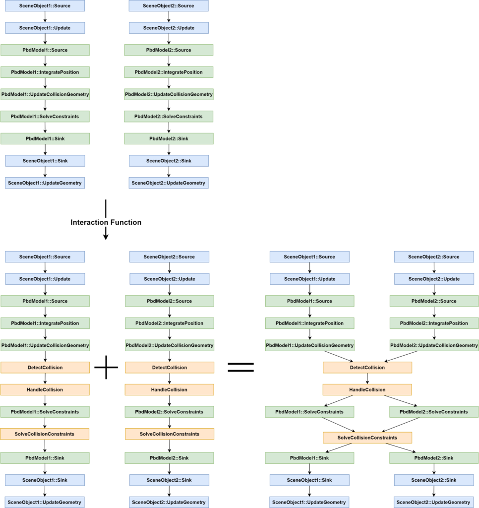
Figure 4: Practical example showing the addition of interaction between two PBD objects. Adding the interaction nodes produces two disconnected graphs that are later fused at initialization.

Critical Task Nodes

Any task added to the task graph may be marked as “critical”. This tells the task graph that it may be accessing shared data and it should be treated as a critical section of code. These are resolved in a preprocessing step available to the task graph, which establishes a directed edge between critical nodes found to be running in parallel. This is often useful in the iMSTK scene when specifying multiple interactions in the same location. The order is not yet guaranteed or specifiable.

Construction of Scene-level Task Graph

Using all these tools, the scene constructs its task graph in three steps. First, it builds the graph. This is done by nesting and summing all of its objects graphs while resolving critical nodes. After the graph is built, a callback is provided for the user to optionally modify the graph. Lastly, the Task Graph  [MD1] is initialized. Here it configures the controller to use, optionally reduces the graph removing redundant edges (transitive reduction) and nodes and optionally writes the results. Additionally,  users may make changes during runtime before or after the scene advances in time allowing them to easily insert, remove, or move steps at any point within the physics pipeline.

Introspection

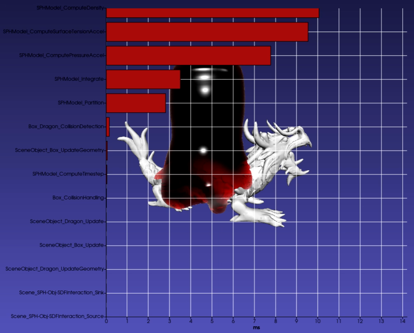
The modular nature of the tasks allows easy introspection capabilities to individual nodes as well as for the entire task graph. The user can request that the graph time each task node to quickly discover bottlenecks. When toggled on, a bar graph showing the computation times for each node of the graph is overlaid on the scene (which uses VTKCharts and therefore works with VTK backend only). The bar graph updates in real-time as the scene steps in time (see Figure 5).

Additionally, the user can find the most time-consuming aspects of the scene. Figure 6 shows in red the critical path (i.e., the path that took the longest to compute) in the scene’s task graph computed using Dijkstra’s algorithm. While this is not meant as a replacement for advanced parallel profilers, it gives users a quick way to see the performance bottlenecks directly in the context of the task graph that is defined. Users may use the imstk::TaskGraphVizWriter to write a GraphViz file which can be drawn by many online tools (webgraphviz, GraphvizOnline).

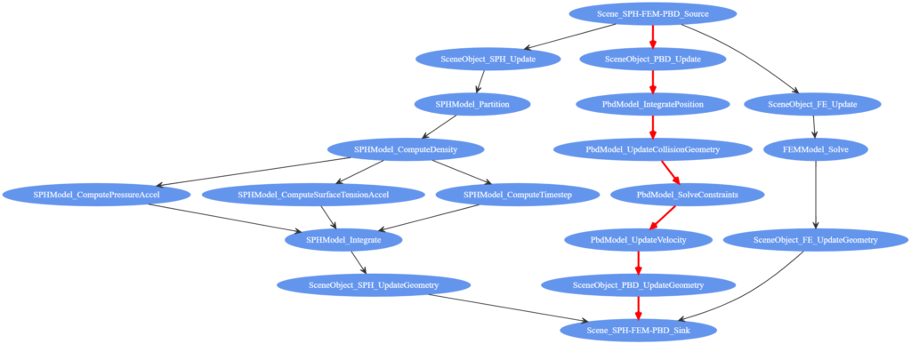
Figure 6: Task graph of an imstk scene with PBD, FEM, and SPH objects with critical path highlighted in red.

Future Work

Performance with the TbbTaskGraphController has often improved for larger scenes (those with more objects). Furthermore, gains were seen in models such as the SPH that are not well loop parallelized, to begin with.

We would like to explore the following directions to extend the capabilities of the current task graph, to broaden its application in iMSTK as well as improve its efficiency.

• Extend TaskGraph to be GPU-compatible, allowing certain task nodes to be marked for GPU dispatch. Extra synchronization nodes may be needed to synchronize data between CPU and GPU.
• Extending the TaskGraph to the imstkModule class which launches its own separate threads (e.g. rendering and devices threads).
• Explore real-time scheduling and provide a mechanism for rationing threads among each task’s loop parallelism. Currently, scheduling is left up to the TBB scheduler.
• Refactor spatial partitioning in collision stages to utilize the flexibility provided by the TaskGraph. Currently, a global singleton is used for spatial partitioning of objects using octrees.

Acknowledgments

The research reported in this publication was supported, in part, by the following awards from NIH: R44DE027595,  1R01EB025247, 2R44DK115332.

Note: The content is solely the responsibility of the authors and does not necessarily represent the official views of the NIH and its institutes.