ParaView HPC Scalability Guide

Context

When deploying ParaView in an HPC environment, once all the technical requirements are met, everything is working perfectly and users start to try and use ParaView for actual data post-processing, one of the first questions that may come to mind is how many cores and nodes should be used by ParaView servers ?

This very simple question has a very complex answer, which depends on many parameters; from the hardware being used, to the type of datasets being processed, or the post processing filters in use.

This blog post will try to answer this question in order for HPC administrators and users to be able to make these decisions and use ParaView to its fullest potential.

In order to figure out how many nodes and cores per node one should use when using ParaView in a distributed environment, many notions will need to be understood and the whole user workflow will need to be evaluated. First, some vocabulary will be necessary.

• Distributed: Distributed execution of a code is when a code is run on multiple nodes or multiple cores, typically using a MPI implementation. Sometimes referred to as parallel.
  
• Distributed Data: When working with a distributed server, ParaView will usually expect the data to be spatially distributed on each server so that each server processes and renders only part of the data.
  
• Headless: Rendering without a graphical environment (like Xorg server), which can use GPU or CPU.
  
• MPI: Message Passing Interface, a node-to-node communication standard used in all HPC, multiple implementations exists, OpenMPI, MPICH and many others.
  
• MultiThread: Parallel execution of a code (on CPU) within a single node, using potentially all the node’s core. Not all ParaView filters support this. MultiThread implementations are typically TBB or OpenMP. Sometimes referred to as SMP.
  
• Pipeline: Series of ParaView filters organised in a direct acyclic graph and executed by ParaView.
  
• pvserver: ParaView server executable, which is usually run with MPI in a HPC environment.
  
• Rendering: Transforming a 3D scene into a 2D image, usually very efficiently performed by the GPU, but not necessarily.
  
  

Evaluate your workflow

In order to be able to answer this question, each user will need to evaluate their workflow and understand what is limiting the workflow and see how to improve it.

User Evaluated slowness

First, while evaluating of existing workflows, a user can see slowdowns of ParaView at different moments. Identifying these moments can be very helpful.

1. Clicking Apply

When a user clicks Apply in ParaView, all non up-to-date filters and readers will be executed and a rendering will be performed. A slow response in this case could be induced by many factors and a refinement of the evaluation will be needed.

2. Stepping in the animation

When a user steps in the animation, all filters and readers dealing with temporal data will be executed and a rendering will be performed. A slow response in this case could be induced by many factors and a refinement of the evaluation will be needed.

3. Interacting with the 3D view

When a user interacts with the view, interactive renders will be performed (by default). A slowness here is probably related to data rendering or network connection.

4. Stopping interaction with the 3D view

When a user stops interacting with the view, a single still render will be performed (by default). A slowness here is probably related to data rendering.

Refining slowness evaluation

If a user’s evaluation of the ParaView’s slowness is already a good piece of information, paraview also provides tools to refine this evaluation in order to make better decisions afterwards.

1. Progress Bar

When executing the pipeline, ParaView’s progress bar will move multiple times from left to right, each time associated with a specific name. If the progress bar is moving slowly at some point, the name on it can be a good indication of what is taking some time. Usually this name is related to a specific filter or reader in the pipeline, or it can sometimes be related to the data rendering (for example: vtkGeometryWithFaces)

2. RenderView annotations

Showing the “RenderView Annotations” could give a good indication of rendering issues and slowness.

Check the Edit -> Settings -> RenderView -> ShowAnnotation setting, to see it appearing.

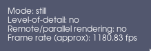
A low framerate is the indication of a slow rendering.

3. TimerLog

The Timer Log gives complete information about the time taken by each part of the process. It is very complete and usually always gives enough insight to understand the source of any slowness issue. You can access it by using
Tools -> TimerLog.

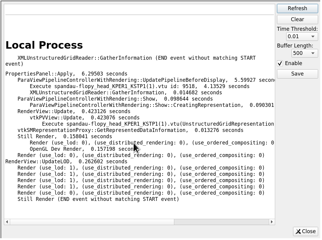
However, it can be hard to read, so here is how to do it.

• First put ParaView in a situation just before the next interaction causes a slowness you would like to evaluate,
• Open the timer log, press Refresh and Clear.
• Do the interaction causing the slowness in ParaView,
• Finally, press Refresh in the timer log, then Save it in a file.

A typical Apply timer log results would look like this:

PropertiesPanel::Apply,  5.05854 seconds
    RenderView::Update,  3.48657 seconds
            vtkPVView::Update,  3.48649 seconds
                   Execute file.vtu id: 9518,  3.11645 seconds
                Execute SurfaceRepresentation id: 9721,  0.360019 seconds
    XMLUnstructuredGridReader::GatherInformation,  0.010803 seconds
    vtkSMRepresentationProxy::GetRepresentedDataInformation,  0.012216 seconds
    Still Render,  0.130475 seconds
            Render (use_lod: 0), (use_distributed_rendering: 0), (use_ordered_compositing: 0)
            OpenGL Dev Render,  0.129251 seconds

The indentation level represents the different steps and which step is part of another step.

Here one can see that:

• The whole Apply took ~5s
• Reading the file took ~3.1s
• Extracting the surface took ~0.36s
• Rendering took ~0.12s

So clearly, someone willing to improve these times should focus on reading the file part, and not the rendering. This is a very simple example and reading this log can get complicated, especially when working with distributed pvserver.

Identifying the limiting factor

With all this information, one should try to identify the limiting factor which may be causing visible slowness. Here are a few possibilities

1. Rendering heavy pipeline

A rendering heavy pipeline is characterized by a low FPS in the annotations and high Render time in the timer log using either interactive or still render depending on the configuration. You may also want to use an external tool like nvidia-smi to evaluate the load of the GPUs.

2. I/O heavy pipeline

A I/O heavy pipeline is characterized by long progress bars for Readers and high timings for Filenames in the timer log. You may also want to use an external tool like iostat to evaluate the I/O load.

3. Network heavy pipeline

A network heavy pipeline is characterized by long wait without progress bar and specific related items in timer log with high timings. It can also be characterized by low FPS in the annotations with small geometries. You may also want to use an external tool like iftop to evaluate the network load.

4. Computation heavy pipeline

A computation heavy pipeline is characterized by a long progress bar for specific Filters and high time in the timer log for Filters. You may also want to use an external tool like htop to evaluate the computational load.

Once the limiting factor has been identified, it can be resolved or worked around, however, a deep understanding of the hardware and the ParaView pipeline is required.

Optimizing for Rendering

Rendering Types

There are many ways to perform rendering in ParaView. Some are used to render as fast as possible, others are used to achieve some specific graphical results, others are used by default as nothing better is possible.

1. Traditional OpenGL/GPU based rendering

This is the simplest and fastest way to perform rendering with ParaView, however it requires access to a GPU and a graphical environment. Rendering can even be faster when using a more powerful GPU and will result in a faster rendering. Using the right GPU driver is also necessary to have the best performance.

2. EGL/GPU based rendering

While a bit more complex to set up than OpenGL rendering, EGL only requires a GPU for rendering and is headless. This is still very fast rendering. Using a more powerful GPU will result in an even faster rendering. Using the right GPU driver is also necessary to have the best performance.

3. OSMesa based rendering

This solution enables rendering on the CPU and does not require (nor use) GPU for rendering. This is a very flexible solution but is orders of magnitude slower than any GPU based rendering. To use only when no GPUs are available.

4. Raytracing

A dedicated method to produce realistic rendering, slower than standard rendering. Optimization for this method will not be covered in this blog.

Switching rendering types is controlled by enabling specific options in the compilation of ParaView. The different ParaView binary releases also provide different rendering types.

The choice between local/remote rendering is controlled by the dedicated settings in Edit -> Settings -> RenderView in ParaView.

Remote Rendering

When connecting to a server and interacting with an actual dataset, ParaView will use remote rendering by default. Remote rendering means that the rendering happens on the server side and not the client side. The resulting image will then be sent to the client but this part is covered in the network part. 

To optimize for a rendering heavy pipeline using non distributed remote rendering, it is only necessary to make sure the right GPU and GPU drivers are being used.

Distributed Remote Rendering

In the context of a distributed server and remote rendering, ParaView will perform distributed remote rendering where each server performs rendering of the part of the dataset it is computing on. This distributed rendering has a significant overhead and will only start to scale by the number of distributed servers once the dataset reaches a certain size and will depend on the way the data is distributed.

When using GPU rendering, each distributed server has access to a GPU to use. In these conditions, with enough GPUs, interactive rendering of a huge dataset can be attained.

When using OSMesa for rendering, there are no GPU constraints but with the rendering being much slower, it can be hard to attain high FPS.

In order to optimize for a rendering heavy pipeline using distributed remote rendering, it is necessary to provide each server with a GPU to use and make sure the right GPU and GPU drivers are being used.

Local Rendering

When connecting to a server and visualizing small datasets, ParaView will perform local rendering. This means that the dataset’s external geometry is sent to the client (instead of only images) and rendered on the client using the client rendering capabilities.

While this is fine for small geometries, transferring a huge dataset between server and client will be very time consuming network-wise and is not recommended. Moreover, when working with distributed servers, it is firstly necessary to reduce the data to a single server, which is even more time consuming.

Do not use local rendering with actual datasets.

The “First” Render

Many users have noticed that the “First Render” can take more time than subsequent render. This is because even once the data is available on the server side, to perform surface rendering, the surface needs to be extracted first. This surface extraction is only performed when needed, hence the concept of first render. Technically, this can be considered as part of the data computation and will be covered in the dedicated section.

Optimizing for network

Client to Server communication

During ParaView’s standard usage connected to a distributed server, the client and main server will need to communicate. First, the client needs to instruct the server how to create the pipeline. The data needed for this communication is fairly small and should not be limiting.

Then the server needs to send results back to the client. When using local rendering, the whole external geometry of the dataset needs to be sent, this can be very costly. When using remote rendering, images need to be sent from the server to the client. This can be costly especially when interacting with the data and can also be limiting.

Network wise, the faster the better, gigabit or infiniband connections between the client and the server would provide enough bandwidth for high FPS. Slower connections may rely on dedicated settings in ParaView (Edit -> Settings -> RenderView -> Image Compression).

In order to optimize for a client/server network heavy pipeline using remote rendering, use the fastest network connection possible and improve image’s compression if needed.

Distributed Server communication

When using distributed servers, servers will be communicating a lot with each other. This communication may be very heavy depending on the filters used in the ParaView pipeline. It is critical to use gigabit or infiniband between nodes to ensure an acceptable performance.

Optimizing for I/O

I/O heavy workflow and memory tradeoff

When working with a ParaView server, the server is responsible for reading the data from the filesystem. Depending on the format in use and the way ParaView is used, there are possible optimizations.

Firstly, binary formats should always be preferred, as these types of file are being read at a much faster pace. Secondly, files should be stored on high bandwidth I/O disks.

In certain cases, ParaView may need to read the same files multiple times, eg. when working with a temporal dataset. This can be avoided by turning the on Edit -> Settings -> General -> CacheGeometryForAnimation, however this may increase ParaView’s memory usage a lot.

In order to optimize for an I/O heavy pipeline use binary file formats, store files on a fast disk and use cache for animation when needed.

Distributed I/O and filesystem

When working with a distributed ParaView server, the data should be distributed. This is usually done by using a format supporting parallel reading of the data. Here is a non-exhaustive list of file formats:

• Parallel VTK Formats: .pvtu, .pvti, .pvtr…
• CFD General Notation System: .cgns 
• XDMF3: .xmf, .xdmf, .xdmf3, .xmf3
• OpenFOAM: .foam (not the most efficient file format here)
• Exodus: .ex2
• ADIOS2: .bp, .bp4
• Ensight: .case

Usually, these files’ data distribution is static with an already determined number of distributed pieces. Reading each piece by one distributed server can be efficient.

Note: Non distributed files can be redistributed using a dedicated filter but this is hardly efficient.

Moreover, the file will be accessed from each distributed server at the same time, so they must be visible from all nodes and should be efficient to read even when accessed by multiple servers at the same time. For this purpose, it is critical to use a filesystem specialized for this task. PVFS or Lustre come to mind.

In order to optimize for I/O heavy pipeline in a distributed context, use distributed file formats on a distributed file system. Matching the number of servers with the number of pieces of the distributed dataset is a good place to start, adjustments may be needed.

Optimizing for computation

Types of computation

There are many filters in ParaView, each of these filters have many options. Depending on the input type and options, different types of computation can happen.

1. Serial Computation

This type of computation is the most common and the most simple. When working in a distributed environment, ParaView will still be able to work with serial computation in a distributed way, as each server will execute the filter independently, using only one thread on the nodes the server is running on.

2. Multithreaded Computation

This type of computation is more complex to implement, so not yet prevalent in ParaView, but it is growing. When executing a multithreaded computation, each server will use all available ressource on the node they are computing on, using multiple threads.

3. Distributed Computation

This type of computation is only implemented when needed by the algorithm. It may imply lots of network communication between the different pvserver. Within distributed computation, the algorithm can then be implemented using multithreaded computation or not.

Serial Computation

Most ParaView filters are using serial computation.

In order to optimize for serial computation filters in a distributed context, use as many pvserver as you have cores across all your available nodes.

Multithreaded computation

Some of ParaView filters use multithreaded computation, especially in the context of UnstructuredGrid datasets. Here is a non-exhaustive list of filter in ParaView 5.10.0 using multithreaded computation:

• WarpByVector
• RessampleToImage
• Calculator
• CellCenters
• CellDataToPointData
• GenerateSurfaceTangents
• Gradient
• PlotOverLine
• ResampleWithDataset
• WarpByScalars
• Animate Modes
• Compute Derivatives
• Deflect Normals
• Elevation
• Gaussian Resampling
• Merge Vector Components
• Redistribute Data Set
• Vortex Core
• Contour: Only with UnstructuredGrid input
• Slice:  Only with UnstructuredGrid input

In order to optimize for multithreaded computation filters in a distributed context, use as many pvserver as you have available nodes. As each node will benefit from the multithreaded computation, this should result in better performance. In order to ensure optimal usage of available threads, be sure to pay attention to the binding pattern used by MPI to associate its ranks to hardware. Running 1 rank per physical CPU that is improperly bound might only use a subset of available threads while the rest of the compute power idles. Check your implementation’s documentation for information on defaults and controlling options (https://hpc-wiki.info/hpc/Binding/Pinning#Options_for_Binding_in_Intel_MPI).

Distributed computation

As stated earlier, distributed computation is performed by filters requiring communication with other servers in their algorithms during the computation. These communications and computations are handled by MPI. The ParaView binary release provides its own MPICH-ABI compatible mpi implementation that you can use. So if you have access to a MPI implementation optimized for your environnement, make sure to use it. If this MPI implementation is MPICH-ABI compatible, you can use the ParaView binary release with it. If not, make sure to use a ParaView built with your own MPI implementation. Building ParaView is not covered by this blog.

In order to optimize for distributed computation, make sure to use the right version of MPI, then refer to the serial or multithreaded section depending on your workflow.

Decision Flowchart

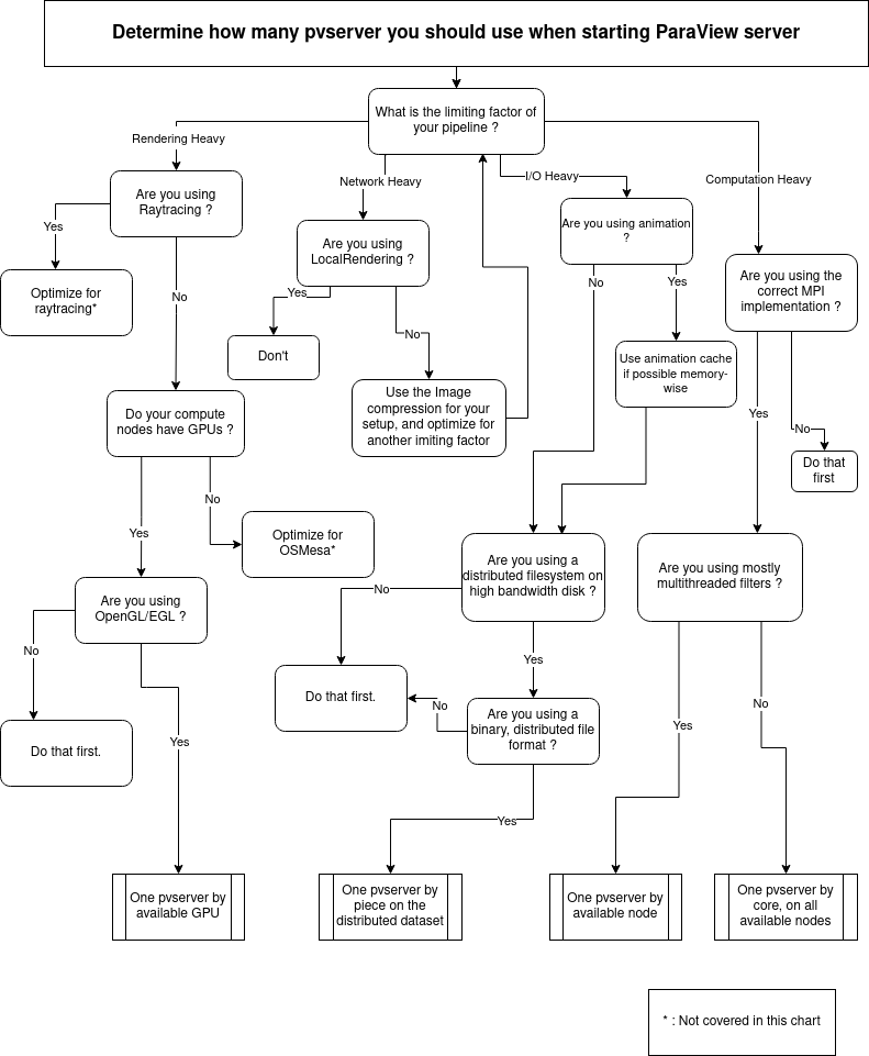
Benchmarking the optimal distribution

Once you have evaluated your limiting factors, the actual optimal distribution of pvserver for a specific workflow may lie in the middle of the suggested optimization. There is no better way to find the right one except by actually benchmarking the different pvserver combination. Here is a set of recommendations for this.

• Run you benchmark in the condition the user will use ParaView in, this include, network setup, other users using shared resources and so on
• Use the timerlog for benchmarking single reader/filter, use pvpython for benchmarking complete workflow
• Alternatively, use pvpython and time module to measure execution times.
• Do not forget to drop file cache before starting a run
• In a HPC environment, first benchmark on a single node with multiple cores, then benchmark on multiple nodes, then readjust the number of cores by nodes

You can also contact Kitware directly for a dedicated help via our support services.

Acknowledgements

This blog was funded by the BAW (www.baw.de).