ParaView’s Python Programmable Filters in Geophysics

With the ability to write data sources and filters in Python code within a ParaView pipeline, we are able to quickly prototype added functionality that our geodynamic scientists are eager to use. This article provides details on the implementation of a selection of these filters as Python programmable filters. Some of the added features are generic enough to be used by other communities of users.
The Visualization Toolkit (VTK) does not have a native spherical grid structure for data based on spherical coordinates (R-, θ-, Φ). Using a vtkStructuredGrid, we are able to maintain a spherical grid structure, enabling volume of interest (VOI) selection for certain radii or for latitudinal or longitudinal subsections.
Geophysics and Climate Related Data
In the study of convection-driven dynamo models in Earth-like planets, the flow in rapidly rotating convection is dominated by columns aligned with the axis of rotation. It is thus naturally more interesting to sample such spherical data with cylinders aligned with the poles. However, it is best to display the data as an unwrapped sheet on a piece of paper. Likewise, the display of constant-radius surfaces such as the outer surface of the Earth is traditionally done with well-known cartographic projections, such as the Mercator, Winkel, or Hammer projections, to cite just a few. We are in luck. VTK includes all of the mappings of the PROJ.4 library [1]. The challenge is to get to the library from ParaView.
We have prototyped sampling spherical data with cylinders and displaying the data as an unwrapped sheet with Python programmable sources and filters.
Cylindrical Sampling
Our driving goal is to use a structured grid, instead of a vtkPolyData object, in order to further manipulate the resampled data using NumPy’s numerous methods of data analysis. To do so, we create a two-dimensional (2D) vtkStructuredGrid at the required sampling resolution and use two copies of the grid.
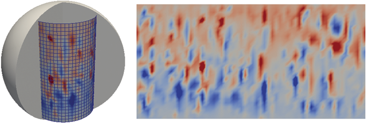
Figure 1: Cylindrical data resampling of the radial component of the magnetic field (Br).
The first one has coordinates wrapped into cylindrical space to sample the output volume, and the second one is a flat sheet for printing. We add the copies of the grid to a vtkMultiBlockDataset structure of a programmable source.
import numpy as np

from vtk.numpy_interface import algorithms as algs

from vtk.numpy_interface \

import dataset_adapter as dsa

executive = self.GetExecutive()

outInfo = executive.GetOutputInformation(0)

exts = [executive.UPDATE_EXTENT().Get(outInfo, i)
  for i in xrange(6)]

whole = [executive.WHOLE_EXTENT().Get(outInfo, i)

for i in xrange(6)]

global_dims = ([whole[1]-whole[0]+1,

whole[3]-whole[2]+1, whole[5]-whole[4]+1])
# first output is the wrapped plane

sg0 = vtk.vtkStructuredGrid()

sg0.SetExtent(exts)

Radius = 0.8

ThetaAxis = np.linspace(-np.pi,np.pi,

global_dims[0])

PhiAxis = np.linspace(-np.pi.5,np.pi.5,

global_dims[1])

xc, zc = np.meshgrid(ThetaAxis,PhiAxis,

indexing="xy")

Xc = Radius * np.sin(xc)

Yc = Radius * np.cos(xc)

coordinates = algs.make_vector(Xc.ravel(),

Yc.ravel(), Radius * zc.ravel())

pts = vtk.vtkPoints()

pts.SetData(dsa.numpyTovtkDataArray(coordinates,

"Points"))

sg0.SetPoints(pts)
# second output is the “flat” plane

sg1 = vtk.vtkStructuredGrid()

sg1.SetExtent(exts)

zc_other = np.zeros(xc.size).reshape(xc.shape)

coordinates = algs.make_vector(xc.ravel(),

zc.ravel(), zc_other.ravel())

pts = vtk.vtkPoints()

pts.SetData(dsa.numpyTovtkDataArray(coordinates,

"Points"))

sg1.SetPoints(pts)

output.SetBlock(0, sg0)

output.SetBlock(1, sg1)
Once the volume is resampled, the 2D array of data can be further processed. For example, we can perform one-dimensional (1D) averages over latitude or longitude. While performing the average can be done with one line of code with NumPy, it takes a few more lines of code to make it happen in ParaView, as we need to create a vtkTable to be able to make a plot in an XYChartView.
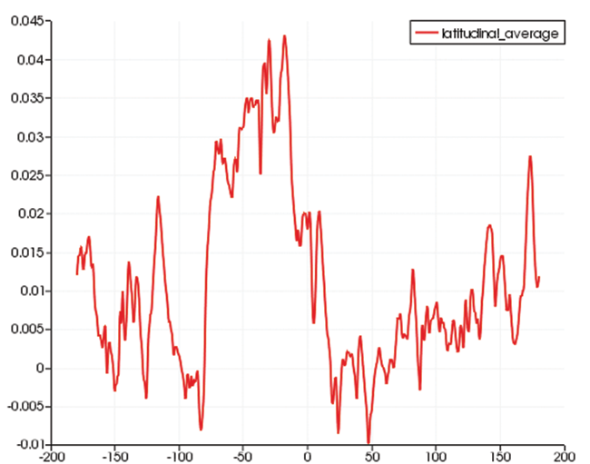
Figure 2: Latitudinal average of Br.
import numpy as np

executive = self.GetExecutive()

outInfo = executive.GetOutputInformation(0)

whole = [executive.WHOLE_EXTENT().Get(outInfo, i)

for i in xrange(6)]

inData = inputs[0].PointData['Br']

data = np.mean(inData.reshape(whole[3]+1,

whole[1]+1), axis=0)
used as X axis for plot
output.RowData.append(np.linspace(-180, 180,
whole[1]+1), "longitude")
output.RowData.append(data, "latitudinal_average")
3D Longitudinal Averaging
NumPy can be used on arrays with multiple dimensions. Using the original three-dimensional (3D) volume’s first meridian slice (0 degrees east longitude), we can display a longitudinal average. The input to NumPy is an NxMxP array. This time, NumPy’s mean will produce a 1xMxP array, which we append to the zero-th slice of the volume in our [Φ, θ, R] space.
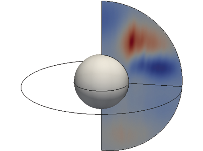
Figure 3: Averaging over the first (longitude) direction.
Spherical Sampling Unwrapped
There are cases when we wish to sample the data on a spherical shell. Some solvers in geodynamics use unstructured grids, and the ability to recover shell-like surfaces is of great interest. We extend our previous sampling by creating a 2D grid at the required sampling resolution. It is wrapped as a sphere for sampling and unwrapped for display.
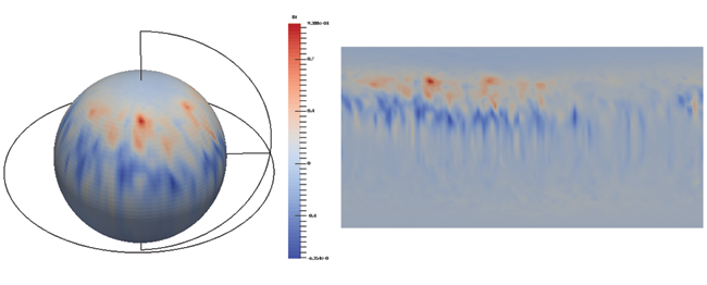
Figure 4: A spherical shell used to sample any grid is flattened for display (from 180 degrees west longitude to 180 degrees east longitude).
2D Cartographic Projections
The outer surface of the Earth is extracted as a VOI, and it becomes an NxMx1 vtkStructuredGrid, which can again be mapped onto a flat sheet of paper. We attach texture coordinates to the grid in order to map photography to the display. Here, we include only a few lines of code with the following core ideas:
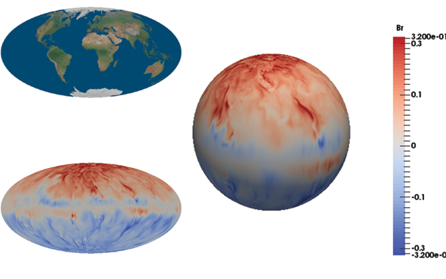
Figure 5: Texture-mapped Earth photography (top left), projected data (bottom left), and 3D spherical data (right) on the core-mantle boundary.
import vtk, vtkGeovisCorePython

from vtk.numpy_interface import algorithms as algs

import numpy as np
# Create a Projection Source

proj = vtkGeovisCorePython.vtkGeoProjectionSource()

proj.SetProjection(ProjectionName['Hammer'])
# Create 1D data arrays for textures and axis

longitude = np.linspace(-180.,180., global_dims[0])

latitude  = np.linspace(-90. ,90. , global_dims[1])

tex_0 = np.linspace(0.,1., global_dims[0])

tex_u = np.tile(tex_0, yres)

tex_1 = np.linspace(0.,1., global_dims[1])

tex_v = np.tile(tex_1, (xres, 1)).T.ravel()

texture_coords = algs.make_vector(tex_u, tex_v)
newPoints = vtk.vtkPoints()

proj.GetTransform().TransformPoints(inPts, newPoints)

output.SetPoints(newPoints)

output.PointData.append(texture_coords,

"TextureCoordinates")

output.PointData.SetActiveTCoords("TextureCoordinates")
Parallel Support
The simulation outputs we use often have resolutions in the range of 100-200 m cells. Implementing a parallel reader is our first priority. Once running ParaView in parallel, we carefully implement our programmable filters to manage the data subdivisions. The filters set the key CAN_PRODUCE_SUB_EXTENT(), and careful indexing (not shown in the source code above for clarity) is used to treat partial results.
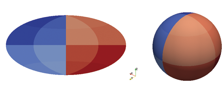
Figure 6: Data subdivision among pvservers.
Summary
We have found the use of ParaView’s programmable filters and sources to be very convenient to prototype new ideas, giving us access to the full VTK Python modules that are available under the hood. Furthermore, combining the strength of NumPy and the ease-of-use of the vtk.numpy_interface package has provided a powerful environment to customize ParaView for different user communities.
We thank Andrew Jackson and Andrey Sheyko [2] of the Eidgenössische Technische Hochschule (ETH) Zürich Institute of Geophysics, who contributed data and motivation for these ParaView developments.
References
[1] Open Source Geospatial Foundation. “PROJ.4 – Cartographic Projections Library.” OSGeo/proj.4. https://github.com/OSGeo/proj.4/wiki.
[2] Sheyko, Andrey. “Numerical investigations of rotating MHD in a spherical shell.” Diss., Eidgenössische Technische Hochschule ETH Zürich, Nr. 22035, 2014.

Jean Favre is the Visualization Task Leader at the Swiss National Supercomputer Centre (CSCS) in Lugano, Switzerland.
@Jean, this is really cool stuff. Thanks for writing this excellent article.
Very impressive article! I use Paraview for solar physics applications (a neighbouring community), mostly for visualizing simulations on rectangular grids. However, I need now to analyse simulations of the solar magnetic vector field on a spherical grid. You mentioned using vtkStructuredGrid for importing exactly that type of data, would you know if there are scripts available for that, or a tutorial accessible to high-level Paraview users explaining how to proceed?
Thank you very much for your help
A spherical grid can be generated with the following code for ParaView5.
# Demonstration script for paraview version 5.0
#
# Creates a spherical grid with a Python ProgrammableSource.
# Works also in parallel by splitting the extents
#
# written by Jean M. Favre, Swiss National Supercomputing Centre
#
# See http://mathworld.wolfram.com/SphericalCoordinates.html
from paraview.simple import *
paraview.simple._DisableFirstRenderCameraReset()
viewSG = GetRenderView()
ReqDataScript = “””
import numpy as np
from vtk.numpy_interface import algorithms as algs
executive = self.GetExecutive()
outInfo = executive.GetOutputInformation(0)
exts = [executive.UPDATE_EXTENT().Get(outInfo, i) for i in xrange(6)]
whole = [executive.WHOLE_EXTENT().Get(outInfo, i) for i in xrange(6)]
global_dims = ([whole[1]-whole[0]+1, whole[3]-whole[2]+1, whole[5]-whole[4]+1])
output.SetExtent(exts)
Raxis = np.linspace(1., 2., global_dims[0])[exts[0]:exts[1]+1]
# only use 3/4 of the full longitude in order to view the inside of the sphere
Thetaaxis = np.linspace(0.,np.pi*1.5, global_dims[1])[exts[2]:exts[3]+1]
Phiaxis = np.linspace(0.,np.pi*1.0, global_dims[2])[exts[4]:exts[5]+1]
p, t, r = np.meshgrid(Phiaxis, Thetaaxis, Raxis, indexing=”ij”)
X = r * np.cos(t) * np.sin(p)
Y = r * np.sin(t) * np.sin(p)
Z = r * np.cos(p)
output.Points = algs.make_vector(X.ravel(),Y.ravel(),Z.ravel())
output.PointData.append(r.ravel(), “radius”)
output.PointData.append(t.ravel(), “theta”)
output.PointData.append(p.ravel(), “phi”)
“””
ReqInfoScript = “””
executive = self.GetExecutive()
outInfo = executive.GetOutputInformation(0)
# A 3D spherical mesh
dims = [3, 9, 7] # radius, theta(longitude), phi(latitude)
outInfo.Set(executive.WHOLE_EXTENT(), 0, dims[0]-1 , 0, dims[1]-1 , 0, dims[2]-1)
outInfo.Set(vtk.vtkAlgorithm.CAN_PRODUCE_SUB_EXTENT(), 1)
“””
programmableSource1 = ProgrammableSource()
programmableSource1.OutputDataSetType = ‘vtkStructuredGrid’
programmableSource1.Script = ReqDataScript
programmableSource1.ScriptRequestInformation = ReqInfoScript
rep2 = Show()
rep2.Representation = ‘Surface With Edges’
Render()
hello – for the 2D cartographic projection section, where you have
proj.SetProjection(ProjectionName[‘Hammer’])
can you ssay how you define ProjectionName — assuming it is a dict that returns an integer corresponding to the projection?
Thanks