Automotive Acoustic Simulation Post-processing with ParaView

April 4, 2024

Kitware note: This is a guest blog from Antonio Baiano Svizzero from Undabit Acoustic Simulations.

Computational Acoustics, particularly when applied using the Finite Element Method (FEM), is a critical tool in various industries such as automotive, aeronautical, building sectors etc. It enables the simulation of sound fields in complex environments, which is essential for optimizing designs for noise reduction and enhancing sound quality.

Car Cabin Modal Analysis with FeniCSx

In this blog post, we present an acoustic modal analysis of a car cabin. Identifying vibration modes that may impact acoustic properties is crucial, as acoustic resonances can amplify noise generated by the engine, a phenomenon often referred to as “booming.” Understanding the frequencies at which resonance occurs and the spatial distribution of the resonant field is essential.

This analysis represents the initial phase of a more comprehensive acoustic simulation that incorporates sources and microphones.

FEniCSx is a popular open source computing platform for solving partial differential equations (PDEs) with the finite element method (FEM). The FEniCSx analysis extracts modes and their shapes to the eXtensible Data Model and Format (XDMF), which can be readily accessed by ParaView.

We propose to describe the step-by-step process to explore and visualize the acoustic modes in ParaView.

Acoustic Mode Visualization in ParaView – Step by Step

The model contains 2 parts:

The car surface model, used for final rendering. It consists of several STL files, and they were kindly provided by Doğukan Uludağ. You can download them here.
The FEniCSx simulation output. This is an unstructured volumetric grid with acoustic fields, within a XDMF file

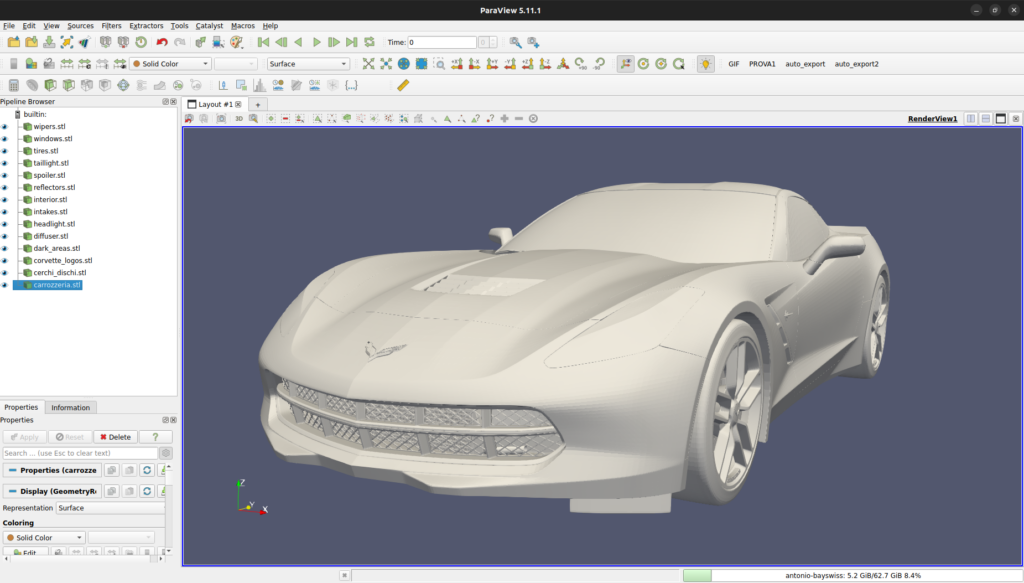
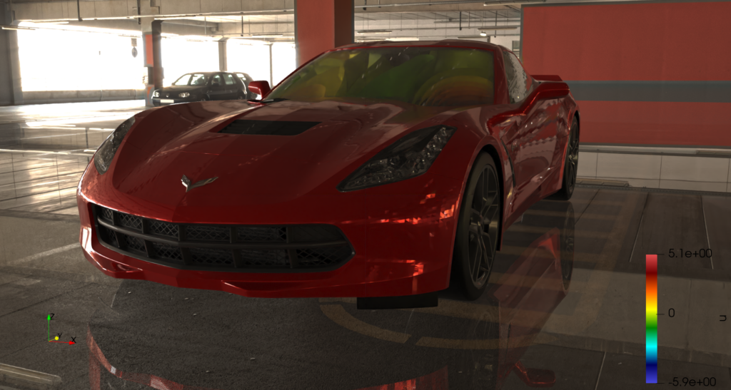
1. Import the car model in STL format

The STL file format is natively supported in ParaView, so using File->Open… menu is enough to get the 3D model displayed in ParaView.

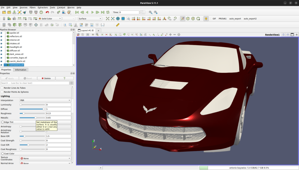
2. Use PBR Lighting interpolation for better rendering

The next step involves adjusting Physically Based Rendering (PBR) parameters to enhance the realism of the car model. This involves refining material properties for each STL subparts to ensure that the model closely resembles to its real-world counterpart.

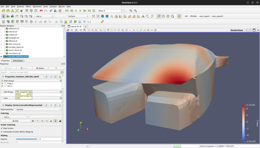
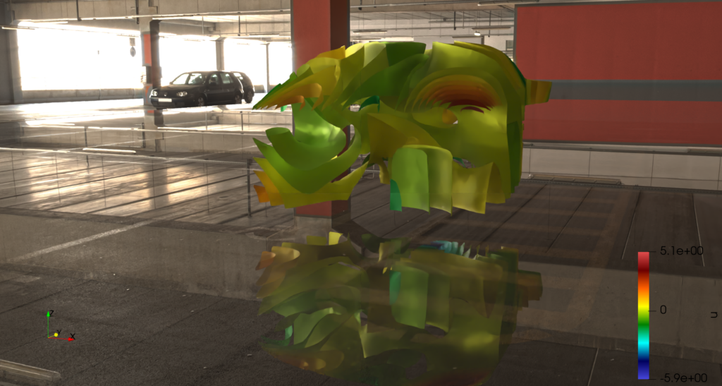
3. Import the FEniCSx Simulation to Display Mode Shape

The imported XDMF file containing the mode shape data, specifically for a 408 Hz mode, is then visualized.

The modes are complex numbers with real parts and imaginary parts and they depend on time. So we need to map these two parts to a double value for visualization at each time step.

For each point in the mesh given a time t, the value could be computed as:

v = Real_part * cos(t) – Imag_part * sin(t).

Thanks to the programmable filter in ParaView, we can compute this value in a dynamic fashion to be updated at each time step. The programmable filter script code is:

real = inputs[0].PointData[0]
imag = inputs[0].PointData[1]

executive = self.GetExecutive()
time_value = executive.GetOutputInformation(0).Get(executive.UPDATE_TIME_STEP())

function = real * cos(6.28 * time_value) - imag * sin(6.28 * time_value)
function_name = inputs[0].PointData.GetArrayName(0).replace('real_', '')

output.PointData.append(function, function_name)

And the Request Information script is:

executive = self.GetExecutive()
outInfo = executive.GetOutputInformation(0)

outInfo.Remove(executive.TIME_STEPS())
for i in range(0, 1000):
  outInfo.Append(executive.TIME_STEPS(), i/100)

outInfo.Remove(executive.TIME_RANGE())
outInfo.Append(executive.TIME_RANGE(), 0)
outInfo.Append(executive.TIME_RANGE(), 1)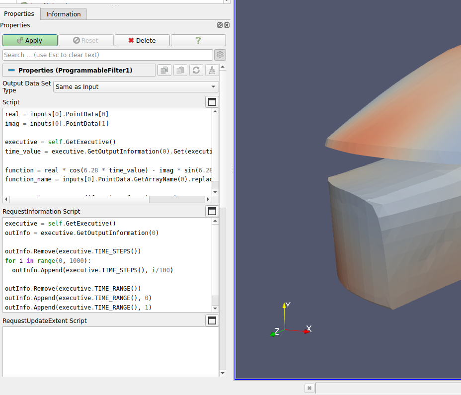

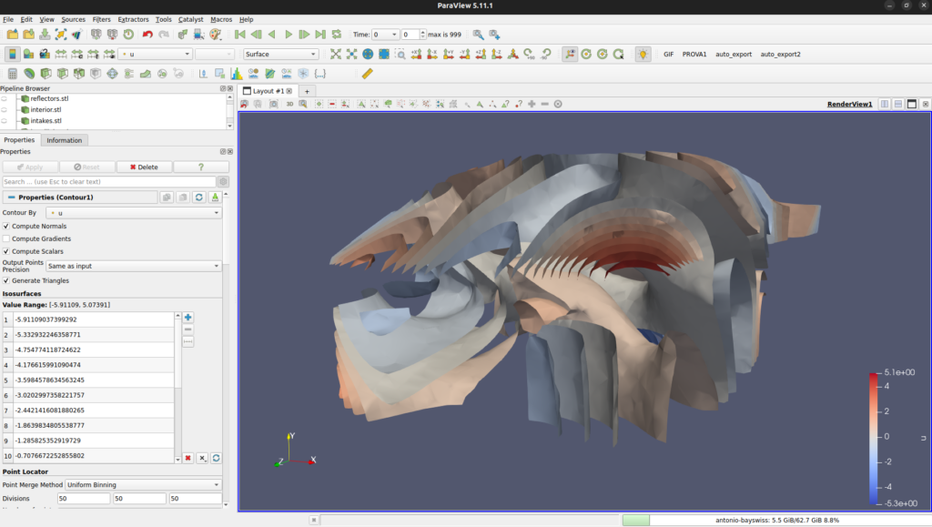
The result is a volumetric data and the default surface representation is not suitable to understand the shape of the wave inside the car. So, we compute 10 contours along the data range to visualize the inner behavior.

Another technique for visualizing the insideof a volume is to use the Volume Rendering in ParaView. You may look at this previous Kitware blog post for the latest developments regarding Volume Rendering:
https://www.kitware.com/volumetric-rendering-in-vtk-and-paraview-introducing-the-scattering-model-on-gpu/

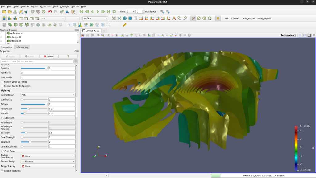
4. Mode shape’s PBR lighting properties

Adjustments to the colorbar and PBR parameters are made to accurately represent the acoustic field within the visualization. This ensures that the representation is both scientifically accurate and visually clear.

5. Setting Up the Camera and Environment

To increase the visual impact of the simulation result, we will prepare a video. Beside the animation of the contour, we will create a camera path which is strategically positioned to capture the essential aspects of the simulation.

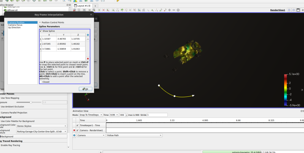
Incorporating a Skybox (downloaded from https://www.ihdri.com/hdri-skies-roofed/) adds a realistic environmental context to the visualization, enriching the overall presentation.

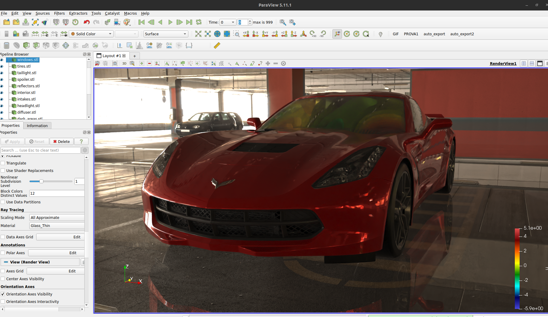
6. Activating Ray Tracing (Intel OSPRay Pathtracer)

In order to achieve photo-realistic rendering, we will switch from the Physically Based Rendering (PBR) to ray tracing. ParaView provides several backends for this purpose like NVidia IndeX or Intel OSPRay.

We activate Intel OSPRay path tracer to introduce advanced lighting and shadow effects, significantly enhancing the realism of the visualization. Parameters are carefully adjusted to balance performance with visual quality.

7. Animation Export

Two distinct scenes are exported: one featuring the car within the acoustic field and another showcasing only the acoustic field. This provides a comprehensive view of the simulation results.

8. Video Editing

The final step involves editing the exported animations to create a cohesive and informative video presentation of the simulation results. This video serves as a valuable tool for analysis, presentation, and documentation purposes.

Conclusion

This article demonstrated how ParaView helped to explore and visualize acoustics simulation from FEniCSx. The flexibility of the programmable filter and the advanced rendering techniques easily emphasize the booming effect for the 408Hz frequency inside the car cabin.

In addition, Paraview is not only useful for this particular resonance phenomenon but is also invaluable for analyzing any 3D acoustic field. It allows for the easy identification of the spatial distribution of sound pressure and nodal planes (areas where the pressure is nearly zero), which is critical for determining optimal locations for resonators or sound absorbers. The clarity in visualizing these elements is not as precise when relying solely on a simple 3D field and slices.

Undabit Acoustic Simulations is an Italian company dedicated to bringing open source simulation to the industry through their advanced expertise in numerical simulation.