Exploratory Climate Data Visualization and Analysis Using DV3D and ParaView in UV-CDAT

In recent years substantial progress in understanding Earth’s climate system is driving an explosion, both in scale and complexity, of climate related data.   Current climate models are capable of generating petabytes of data from a single run.  The complexity of these datasets is also increasing as models encompass an increasingly wide range of earth systems, adding many new variables to the datasets, and requiring integration of an increasingly wide range of observational data sources.

The knowledge discovery process in climate science requires effective tools to discover, access, manipulate, and visualize the datasets of interest.  Recent developments are driving the need for a new generation of climate knowledge discovery tools as the scientists’ traditional toolkit is becoming overwhelmed and rendered obsolete by the “data tsunami”. Key technical challenges include the seamless integration of advanced exploratory visualization tools, workflow and provenance support, and high performance computing.

To address these technical challenges, researchers at NASA, LANL, and Kitware have been developing sophisticated climate data visualization and analysis capabilities as part of the UV-CDAT framework. In the next few sections, we will describe various visual data exploration and computational features provided by DV3D, a package developed at NASA, and ParaView as part of UV-CDAT framework.

The DV3D Package
Graphical representations are very effective at summarizing complex datasets while exposing unusual features. Interactive three-dimensional views into high dimensional datasets can offer a widened perspective and a more comprehensive gestalt, facilitating the recognition of significant features and the discovery of important patterns. The climate knowledge discovery process typically involves complex workflows integrating numerous analysis and visualization processes with many intermediate and final data products.   Workflow systems have been shown to be an effective tool for addressing the challenge of combining disparate computational modules while transparently automating provenance collection [1,2].

DV3D is a VisTrails [4] package of high-level modules for UV-CDAT, providing user-friendly workflow interfaces for advanced visualization and analysis of climate data at a level appropriate for scientists (Figures 1 & 2).  It incorporates numerous features specifically designed for climate data analysis.   It builds on VTK [7], an open-source, object-oriented library for visualization and analysis. DV3D provides the high-level interfaces, tools, and application integrations required to make the analysis and visualization power of VTK readily accessible to users without exposing details such as actors, cameras, renderers, and transfer functions.  It can run as a desktop application or distributed over a set of nodes for hyperwall or distributed visualization applications.

DV3D Plot Types
The DV3D package offers scientists a set of coordinated, interactive 3D views (i.e. plots) into their datasets.   Each DV3D plot type offers a unique perspective by highlighting particular features of the data.  Multiple plots can be combined synergistically (within a single cell or across multiple cells) to facilitate understanding of the natural processes underlying the data.  For example, the plot types include:

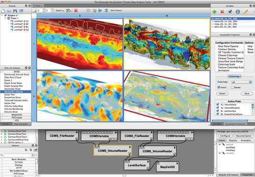Figure 1: DV3D within the UV-CDAT GUI

The Slicer plot provides a set of slice planes that can be interactively dragged over the dataset.   A slice through the data volume at the plane’s location is displayed as a pseudocolor image on the plane.   A slice through a second data volume can also be overlaid as a contour map over the first.  This tool allows scientist to very quickly and easily browse the 3D structure of the dataset, compare variables in 3D, and probe data values.

The Volume Render plot maps variable values within a data volume to opacity and color.   It enables scientists to create an overview of the topology of the data,  revealing complex 3D structures at a glance.  Due to the complexity of creating useful transfer functions, the art of generating volume renderings has in the past been relegated to visualization professionals. DV3D offers interfaces that greatly simplify this process, enabling interactive volume rendering to play an important role in the scientist’s data exploration process.

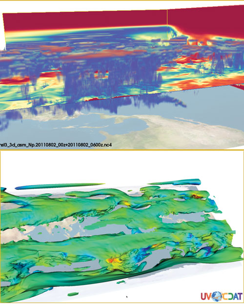Figure 2.  An isosurface plot (bottom) and a combination volume render and slicer plot (top)

The Isosurface plot displays an isosurface derived from one variable’s data volume and colored by the spatially-correspondent values from a second variable’s data volume.  It can produce views similar to a volume rendering while facilitating the comparison of two variables.

The Hovmoller plots are similar to the 3D slicer and volume render plots described above except that they operate on a data volume structured with time (instead of height or pressure level) as the vertical dimension.  This plot allows scientists to quickly and easily browse the 3D structure of spatial time series.

The Vector Slicer plot provides a set of slice planes that can be interactively dragged over a vector field dataset. A slice through the field at the plane’s location is displayed as a vector glyph or streamline plot on the plane.  This plot allows scientists to browse the structure of variables (such as wind velocity) that have both magnitude and direction.

DV3D Plot Features
The plot types described above offer the following features:

• Animating over one of the data dimensions (typically time).
• The VisTrails workflow interface to enable climate scientists to develop custom visualization and analysis pipelines.
• A rich selection of interactive query, browse, navigation, and configuration options facilitating exploratory
• visualization.
• Integration with the VisTrails spreadsheet, which provides multiple, synchronized plots for desktop or hyperwall.
• Integration with the VisTrails provenance architecture to provide transparent collection and comprehensive management of workflow and data provenance.
• The underlying VTK architecture provides active and passive 3D stereo visualization support.
• Seamless integration with CDAT’s climate data management system (CDMS) [8] and other climate data analysis tools to provide extensive climate data processing and analysis functionality.

The DV3D Interface
The DV3D package is composed of a set of VisTrails modules.   Each DV3D module offers a distinctive GUI interface (accessible from the VisTrails workflow builder), enabling the configuration of workflow parameters. These modules can be selected from a palette and linked to create custom workflows using the VisTrails workflow builder.   The DV3D spreadsheet cells also offer a wide range of interactive key-press and mouse-drag operations, facilitating the configuration of colormaps, transfer functions, and other display and execution options.  For example, pressing a button in a configuration panel and then clicking and dragging in a spreadsheet cell displaying a DV3D volume render plot initiates a leveling operation that controls the shape of the plot’s opacity or color transfer function.   The volume render plot changes interactively as the user drags the mouse around the cell.

All configuration operations are saved as VisTrails provenance.  The provenance trail contains a record of all workflow construction and configuration operations that contributed to the current visualization, making it easy to revert to an earlier configuration of the workflow at any stage of development.

DV3D Workflows
A DV3D workflow begins with a set of modules encapsulating CDMS operations for accessing and processing climate data from the local file system, the Earth System Grid Federation, or the ParaView server on a remote supercomputer. The CDAT toolkit provides a wide range of climate data analysis operations, including simple arithmetic operations, regridding, conditioned comparisons, weighted averages, various statistical operations, etc.  A DV3D translation module converts the processed CDMS data volumes into VTK image data instances to initialize the visualization branch of a DV3D workflow.  DV3D visualization modules encapsulate complex VTK pipelines with numerous supporting objects such as actors, cameras, renderers, interaction observers, data mappers, and transfer functions. Each visualization pipeline implements a unique interactive 3D plot. Each branch of a DV3D workflow terminates in a DV3D cell module, which represents a custom cell in the UVCDAT spreadsheet. 

The DV3D cell module includes a configurable base map, navigation controls, onscreen dataset and variable labels, a pick operation display, and legend/colormap displays.  Cells in the spreadsheet can be individually activated or deactivated by selection.  Configuration and navigation operations are propagated to all active cells.

ParaView Plots and UV-CDAT Spatio-Temporal Parallel Pipeline
The integration of ParaView into the UV-CDAT framework has brought a wealth of analysis and visualization capabilities to the framework. The serial abilities of ParaView have been tightly integrated into UV-CDAT, which brings with it several benefits. The parallel capabilities of ParaView can also be accessed by the user using a set workflow. A new addition to ParaView is the calculation of the Meridional Overturning Circulation (MOC) and Meridional Heat Transport (MHT). Also, in response to the demands and use cases of the UV-CDAT program, a new parallel pipeline has been developed to take advantage of temporal parallelism, called the UV-CDAT spatio-temporal pipeline.

Tight Coupling with Serial ParaView and UV-CDAT
UV-CDAT uses VisTrails as its provenance engine and several steps have been taken to tightly integrate ParaView with VisTrails. Several ParaView-specific VisTrails modules have been created including PVContourRepresentation and PVGenericCell, which support one-or-more representations for its input. A ParaView pipeline helper assists in building the plot pipeline and creating instances of ParaView modules. The main benefit of this tight integration between ParaView and VisTrails is the fact that when ParaView plots are used in UV-CDAT, VisTrails automatically collects provenance information about the plots, which can then be shown in the pipeline viewer. Figure 3 illustrates a ParaView plot in UV-CDAT, and the corresponding VisTrails pipeline workflow for that plot.

ParaView is a general-purpose analysis and visualization framework that encompasses users from many scientific fields. UV-CDAT, though, is focused primarily on climate data. Therefore, a simpler, domain-specific interface was created that exposed the features of ParaView that are most useful to the climate community. This includes such visualizations as contour plots and colormap plots.

Several new climate-specific readers and filters have been implemented in ParaView for the UV-CDAT framework. These include an Unstructured POP reader, an MOC and MHT reader, and a Project Sphere filter. The Unstructured POP reader loads POP Ocean data as an unstructured grid. Better analysis and visualizations can be obtained from this more accurate representation of the data. The MOC and MHT reader will be discussed in detail in a later section. The Project Sphere filter takes data defined on a spherical grid, like climate data, and projects it onto a flat plane.

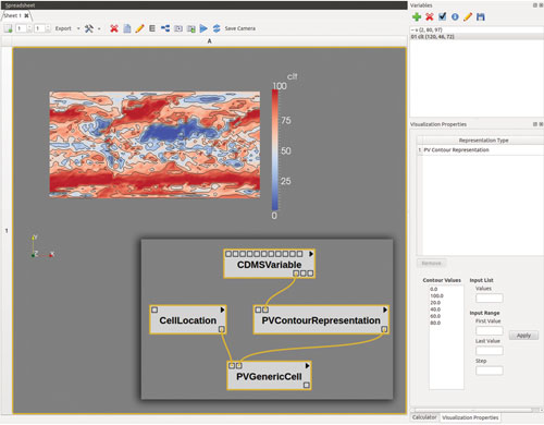Figure 3: ParaView plot and corresponding VisTrails pipeline workflow

Meridional Overturning Circulation and Meridional Heat Transport
The Meridional Overturning Circulation (MOC) and the Meridional Heat Transport (MHT) are two quantities considered important to the analysis of Earth’s ocean currents. Changing the temperature of ocean currents will affect its density, causing it to increase or decrease in depth. In general, ocean currents will heat up and rise near the equator, and will cool down and sink near the poles. The amount of overturning of the ocean currents is referred to as the Meridional Overturning Circulation. The MHT is the transport of heat through ocean currents from the low latitudes near the equator to the high latitudes towards the poles.

Serial programs were first used to compute these two quantities. As the size of the generated data became ever larger, the time required to compute them became too prohibitive, and they were dropped as part of the standard diagnostics. To remedy this, two parallel filters were created in ParaView and integrated in UV-CDAT, which calculate the MOC and MHT in parallel. The performance gains from parallelizing these computations were substantial, with run times being reduced from a couple of hours to a few minutes.

UV-CDAT Spatio-Temporal Parallel Pipeline
Many climate datasets have, in addition to a high spatial resolution, a high temporal resolution. In many instances, simulations output daily or monthly averages, with datasets possibly covering a total timespan of decades.  Due to this high temporal resolution, there is a critical need to have a fast, scalable method for processing a large number of timesteps. In response, the UV-CDAT spatio-temporal pipeline was devised to solve UV-CDAT Use Case 1 and Use Case 2.

Use Case 1
Use Case 1 involves a dataset with high spatial and temporal resolution. The task is to produce an image sequence of the dataset by producing one image per timestep. One key aspect here is that there are no dependencies between timesteps, and each timestep can be processed independently.

In a fully data-parallel model, all available processors would take part in reading the first timestep, perform any required analysis, and then take part in producing the final image output. Then all processors would load the second timestep, and the cycle repeats until all timesteps have been processed. In this case, timesteps are accessed sequentially, and only spatial parallelism is utilized.

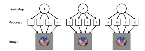
Figure 4: Use Case 1 – High spatial resolution, high temporal resolution, image sequence production

In a fully data-parallel model, all available processors would take part in reading the first timestep, perform any required analysis, and then take part in producing the final image output. Then all processors would load the second timestep, and the cycle repeats until all timesteps have been processed. In this case, timesteps are accessed sequentially, and only spatial parallelism is utilized.

In the UV-CDAT spatio-temporal pipeline, parallelism is extended both spatially and temporally. This means that multiple timesteps can be processed simultaneously. This is permissible since each timestep can be processed independently of each other. In order to achieve temporal parallelism, the available processors are divided into groups called time compartments. The number of total time compartments is dependent on the number of processes and the size of a time compartment, which is constant over all time compartments. Each time compartment can now load and process a timestep independently of each other, resulting in multiple timesteps being worked on simultaneously. Figure 4 illustrates how processors are broken up into time compartments, and how work is distributed among them. When there are more timesteps than time compartments, the files are assigned in round-robin fashion to time compartments, so it is possible for a time compartment to process multiple timesteps. Within a time compartment, its’ assigned timesteps are processed one at a time.

The amount of temporal parallelism versus spatial parallelism is controlled by the size of one time compartment, which is a user configurable parameter. When the time compartment size is large, there are fewer total time compartments, which results in less temporal parallelism and more spatial parallelism. On the other hand, if the time compartment size is small, there are then more time compartments, and the amount of temporal parallelism is higher, the amount of spatial parallelism decreases.

Use Case 2
Similar to Use Case 1, Use Case 2 also involves analyzing climate data, which has both high spatial and temporal resolution. The difference with Use Case 1 is that instead of having each timestep be processed independently, some type of reduction operation among several timesteps must be performed, with the output being various statistics. One example would be calculating yearly averages from monthly data. In this case, every 12 timesteps comprising of one year must be averaged together. Supported reduction operations include average, min, max, and standard deviation.

The UV-CDAT spatio-temporal pipeline can also be used to support Use Case 2, as illustrated by Figure 5. Each time compartment loads one-or-more timesteps like before, but with an additional reduction step, which combines the results of several time compartments into a single data product.

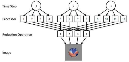Figure 5: Use Case 2  – High spatial resolution, high temporal resolution, time average

UV-CDAT Spatio-Temporal Pipeline Performance
Initial results from the UV-CDAT spatio-temporal pipeline’s performance show vast performance gains. In Use Case 1, there was an improvement from hours to minutes when switching to the spatio-temporal pipeline. Use Case 2 also showed an order of magnitude improvement when using the spatio-temporal pipeline. Similar results have been shown over multiple supercomputers and multiple file systems.

Conclusions
The inundation of data generated by ever-increasing resolution in both global models and remote sensors is presenting both a challenge and an opportunity for earth science analytics. New tools and methods are needed to reap the benefits of this overabundance of information. Key technical challenges include the seamless integration of advanced visualization tools, workflow and provenance support, and high performance computing.

The complexity of the climate knowledge discovery process is increasing due to the increasing complexity of climate datasets.  Graphical representations (which are very effective at addressing data complexity) can be enhanced by an increase in the number of “degrees of freedom” in the visualization process.  Three-dimensional views into complex high dimensions datasets can offer a widened perspective and a more comprehensive gestalt facilitating the recognition of significant features and the discovery of important patterns.

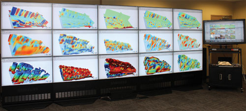Figure 6.  The DV3D distributed visualization framework deployed on the NASA NCCS hyperwall.

Acknowledgment
Resources supporting this work were provided by the NASA High-End Computing (HEC) Program through the Center for Climate Simulation (NCCS) at Goddard Space Flight Center. We would like to thank Dean N. Williams, Berk Geveci, Gerald Potter, and entire UV-CDAT team for this work.

Authors
Many thanks to Thomas Maxwell of NASA; John Patchett and Boonthanome Nouanesengsy of Los Alamos National Laboratory; and Andy Bauer and Aashish Chaudhary of Kitware for contributing this article!

References

1. S. Davidson and J. Freire, “Provenance and Scientific Workflows: Challenges and Opportunities” ACM SIGMOD, pp. 1345-1350, 2008.
2. C. Silva, J. Freire and S. Callahan, “Provenance for Visualizations: Reproducibility and Beyond”, IEEE Computing in Science & Engineering, vol. 9(5), pp. 82-29, 2007.
3. Maxwell, T, DV3D documentation:  http://portal.nccs.nasa.gov/DV3D/, 2010.
4. D. Williams, “Ultrascale Visualization – Climate Data Analysis Tools”, http://climatemodeling.science.energy.gov/projects/ultrascale-visualization–climate-data-analysis-tools-uv-cdat, 2010.
5. S. Callahan, J. Freire, E. Santos, et al., “VisTrails, Visualization meets Data Management”, Proceedings of ACM SIGMOD: 2006. 
6. D. Williams, 2007, “The PCMDI Software System: Status and Future Plans of CDAT (Climate Data Analysis Tools)”, PCMDI Report No. 44. http://www2-pcmdi.llnl.gov/cdat.
7. W. Schroeder, K. Martin, and B. Lorensen, Visualization Toolkit: An Object-Oriented Approach to 3D Graphics, 4th Edition. Kitware:  2006.
8. R. Drach, P. Dubois, and D. Williams, 2007: Climate Data Management System, version 5.0, http://www2-pcmdi.llnl.gov/cdat/manuals/cdms5.pdf.