A Common Pathology Task

In this post, we show how to use foundation models—powerful AI tools trained on vast image datasets—to find and compare structures like glomeruli in kidney tissue. We’ll demonstrate how to integrate these models into HistomicsTK and evaluate their effectiveness for real-world pathology use cases.

HistomicsTK is Kitware’s open-source platform for analyzing histology Whole Slide Images (WSI).  These large images, often multiple gigapixels in size, are cross sections of biological tissue, such as from biopsies.  A core task in pathology is identifying similar regions within an image to determine whether a feature is representative or unusual.

Foundation Models: Powerful Tools

Foundation models are a core building block in the modern AI world.  They are trained on large, diverse data sets to capture features without regard to a specific problem, allowing them to generalize across data domains and tasks.  They can also be adapted for specific applications without complete retraining, making them an attractive starting point for custom models (read about “transfer learning” to learn more about this).

Among foundation models, image embedding models are especially useful as they convert an image into a numerical vector, making it possible to compare similarity across different regions or images.  While powerful, not all foundation models are equally effective for pathology.  HistomicsTK makes it simple to integrate and compare them.

Packaging Models for Use in HistomicsTK

As a first step, we can package any image embedding model so that it can be used from HistomicsTK.  See https://github.com/DigitalSlideArchive/histomicstk-similarity for an example of how this can be done.

HistomicsTK can run any algorithm packaged as a Docker image (or Podman, or Apptainer) and using the Slicer CLI Execution model protocol for specifying inputs and outputs.  This involves wrapping an algorithm in a container with all of its dependencies and adding a small amount of metadata to say what it can do.  These containerized tasks can be simple (e.g., just taking file inputs and generating file outputs), or they can tie tightly into the HistomicsTK API.

In our example, we read any WSI file that can be read by the large_image library.  This is important as WSI files can come in hundreds of nuanced formats, and it is useful to separate the concern of reading these images from the algorithm that we want to use.

Choosing a Model

We can easily use a wide range of models.  We made a simple Python class that abstracts any image embedding model to two parts: loading the model and generating a vector embedding of an image.

We can download such models from common sources, such as huggingface.co.  Some models require authentication or have restrictive licenses.  Some models are general, trained on images without a specific focus on pathology, while others are tuned for pathology but with different training set sizes.  We show off how to integrate three different models (but others are straightforward to integrate as well):

• Gigapath (Apache-2 license): “A whole-slide foundation model for digital pathology from real-world data”
• DinoV2-large (Apache-2 license): “The Vision Transformer (ViT) is a transformer encoder model (BERT-like) pretrained on a large collection of images in a self-supervised fashion.”
• Midnight-12k (MIT license): “Training state-of-the-art pathology foundation models with orders of magnitude less data.”

These represent a range from general purpose (DinoV2) to highly specialized (Gigapath).

Installation

Installation instructions are available in the GitHub repository. This includes how to download the Docker container and how to configure model caching in HistomicsTK to avoid excessive model downloads.

An Example Use Case: Finding Glomeruli

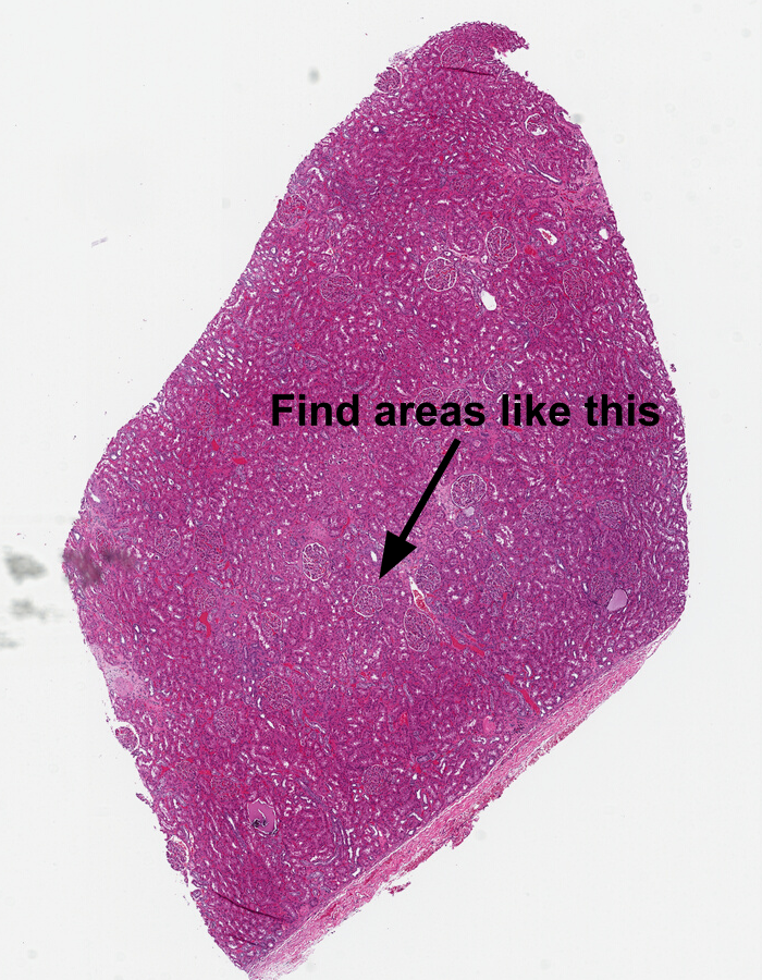
As an example use case, we’ll be looking at a kidney tissue sample from the TCGA.  We picked a normal tissue sample (non-cancerous) with some clear features.

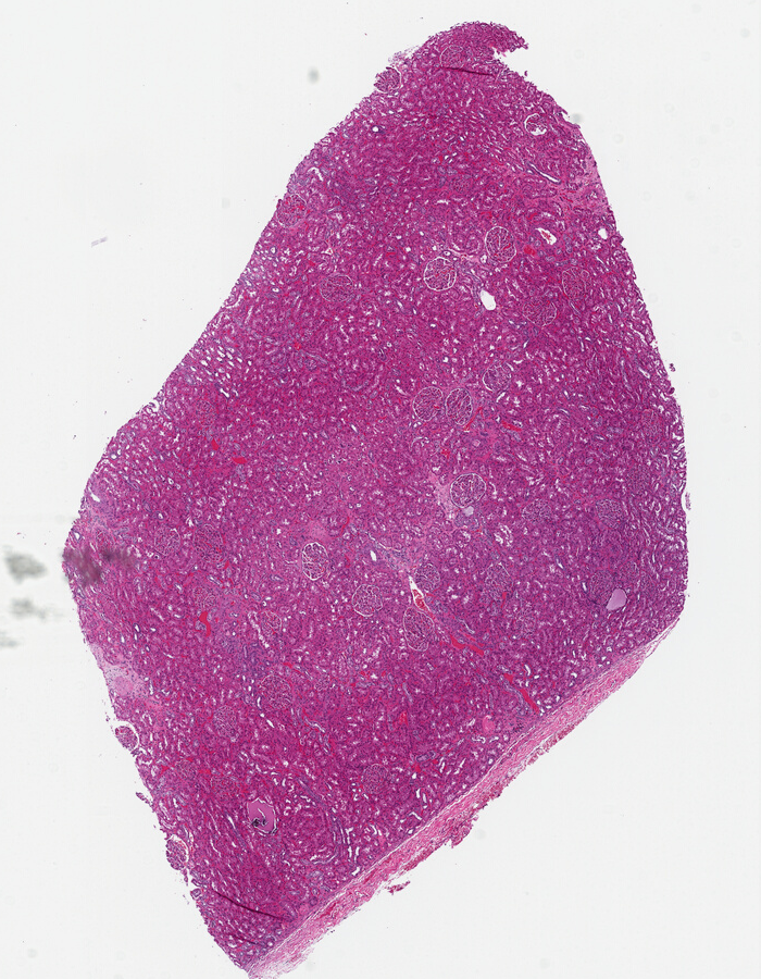
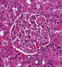
For instance, we might want to find all of the glomeruli.  Even someone who isn’t a trained pathologist can spot these — they are fairly round objects with a distinct texture and often a clear area surrounding them.  As glomeruli are three-dimensional, some are naturally sampled close to their maximal cross section while others are nearer one extreme of the spherical extents.

Calculating our Embeddings

Our analysis will consist of two parts for any given foundation model.  The first part is to calculate the embedding vector for our original image.  Our algorithm divides the WSI into square regions, ideally at the same magnification and image sizes the model was trained on.  For all of our sample models except DinoV2, this is 20x (shorthand for “0.5 µm per pixel”) and 224 x 224 pixels, corresponding to square image patches that are 112 μm on a side.  Any feature much smaller than this is unlikely to be distinguished, while larger features can be found by taking an average of the vector embedding for a small array of patches.

So that we don’t miss features, we can analyze overlapping regions of the image.  By default, our algorithm is set up to work on 224 x 224 pixel images, striding across the whole image at intervals of half that (112 pixels).

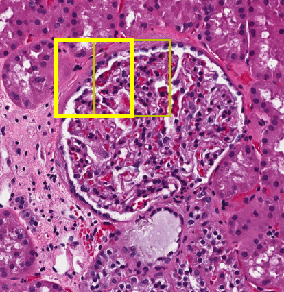
Our example use case will be trying to find glomeruli, which are often in the 150 μm to 250 μm size range, so we know that combining a 2×2 set of image patches without overlap or a 3×3 set with 50% overlap is appropriate.  You’ll see this is a parameter in our task that we could change.

To actually calculate our embeddings we will follow these steps:

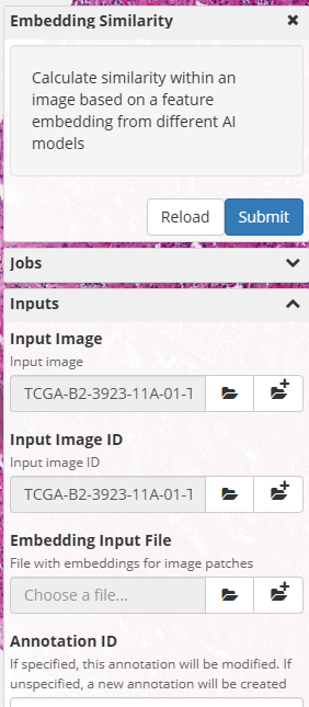
• Open our sample WSI in the HistomicsTK interface
• Select the Analyses -> dsarchive/histomicstk_similarity -> latest -> EmbeddingSimilarity task
• Pick our model
• Adjust stride and other parameters as we see fit (we will use the defaults for this example)
• Pick a better output file name and location so we can remember what we’ve generated (our embedding files are simple numpy compressed files with a .npz extension)
• Click “Submit”

Depending on the size of our WSI, our disk I/O speed, and the speed and quality of our GPU, this will take some time (on this image, using the Gigapath model, an Nvidia Quadro RTX 5000 took around 5 minutes).

Finding Similar Tissue

Once the embeddings for a particular model and image are computed, we can use them to search for image similarity quite quickly (without even involving the GPU)..  These embeddings contain the vector for each image patch, along with metadata recording the stride and other parameters used to generate them.

Assuming we still have our sample image open and the Embedding Similarity task selected, we can:

• Select our embedding file for the “Embedding Input File”
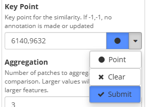
• Turn on auto-submit for the Key Point
• Click the Dot control for Key Point and pick any of the glomeruli

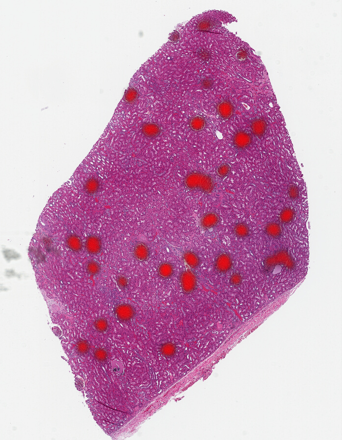
If we are using the Gigapath model, in a few seconds, you’ll see all the glomeruli nicely lit up in yellow on our output heatmap:

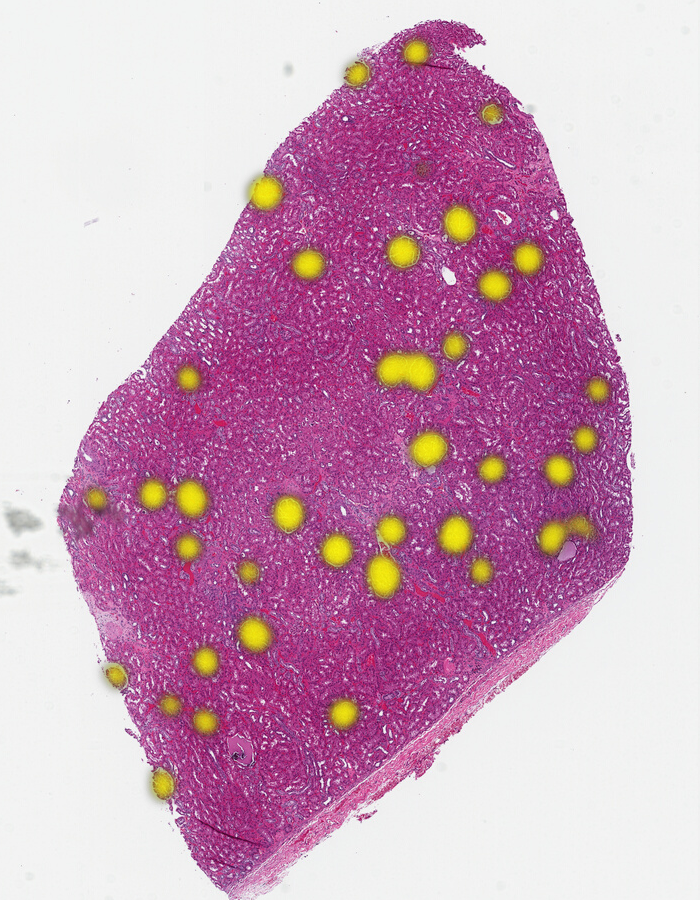
Each time we click, we generate another heatmap.  You can ask to replace the current heatmap by specifying the ID of the heatmap annotation in the task (see the video on the HistomicsTK Similarity repo).

Gigapath versus DinoV2

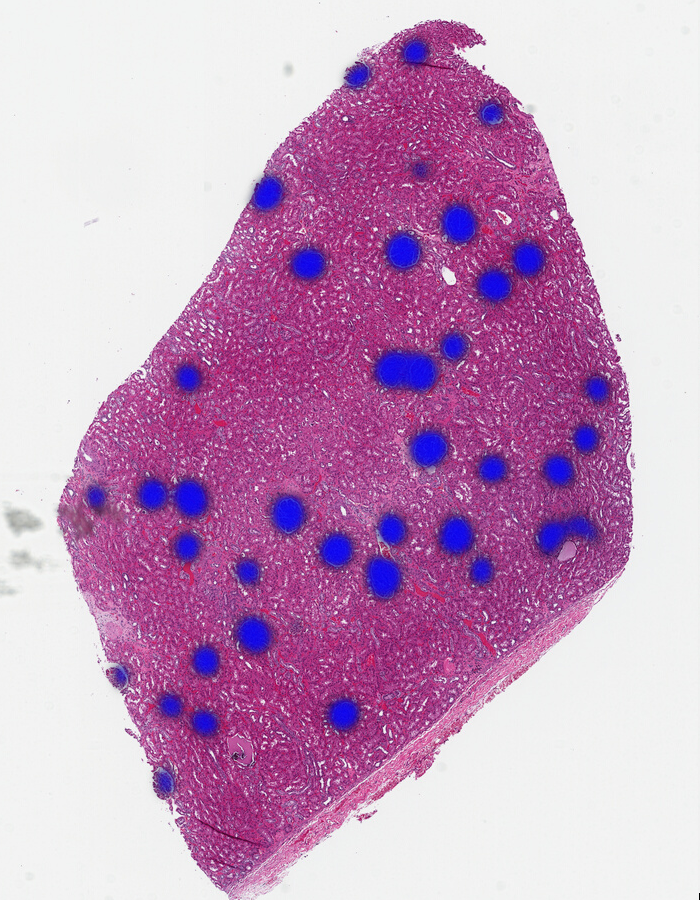
We can try this with a different model: DinoV2.  We’ll change the color in the task settings to red for DinoV2 so we can easily see how it compares.

This initially looks terrible — we didn’t find just the glomeruli, we found almost all of the tissue.

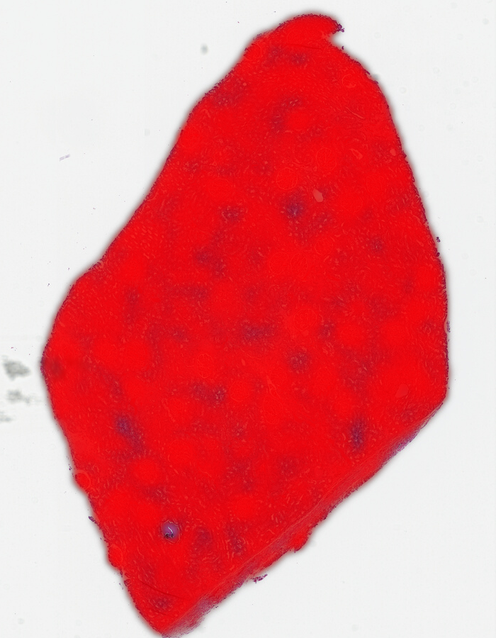
BUT…

One parameter in our task is the Plot Threshold.  We are using cosine similarity to see which areas are the same.  If two embeddings are identical, the cosine similarity will be 1.  If images were as different as possible, it would be -1.  Our plot threshold says that any value less than the threshold is “no match”, and the remaining values are scaled from transparent to full color.  Our default plot threshold is 0.75, which worked well in Gigapath.

Change the plot threshold to 0.96 and try again with DinoV2:

That looks pretty good. It missed some of the glomeruli near the edge of the tissue and overemphasized a region on the right it probably shouldn’t have, so it still isn’t as good as Gigapath at finding glomeruli, but it is still impressive for a non-pathology-specific model.

That the cosine similarity requires such a high threshold shows that DinoV2 has fundamentally less distinction in its feature space for this type of image than Gigapath does.  This shouldn’t be surprising, but if you are training your own adapted model, this might be a perfectly good place to start.

One more Comparison

We’ll show one more model.  This is Midnight with a threshold of 0.93.  It found the edge glomeruli that Gigapath had found, so it has outperformed DinoV2, but, based on the threshold, still has less distinction than Gigapath.

You can see the differences more clearly if we use the same color and alternate between them:

From this you can see Gigapath has more distinction at the tissue edges and a bit better resolution in some areas, while Dino misses the edges and finds some spots to be similar that aren’t glomeruli.  Midnight is substantially better than Dino, but still has less confidence near edges.

You can look at this data yourself here: https://demo.kitware.com/histomicstk/histomics#?image=687e6b34b68a9cab242f2d9a (a free account is required).

Conclusion

Foundation models have shown astonishing success at a wide range of tasks, and they make a powerful starting point for histological image analysis. HistomicsTK makes it easy to experiment with different models and determine what works best for your specific biological questions. If you need help with tuning models, developing an AI-based workflow for your data, or any other question about how best to use HistomicsTK, please get in touch!