Modeling Arbitrary-order Lagrange Finite Elements in the Visualization Toolkit
Two techniques that are used by simulations are geometric refinement (also known as hierarchical refinement, or h-refinement) and polynomial refinement (also known as p-refinement). Traditional simulations often apply geometric refinement, which splits cells with low accuracy to resolve finer spatial features. More recent finite element simulations may also apply polynomial refinement. This technique enhances existing cells, so they can fit a higher-order polynomial to the simulation solution. As a result, the cells can represent more complex functions.
Cells that experience polynomial refinement have an order greater than one. For many years, the Visualization Toolkit (VTK) has handled different orders with different cell types. More specifically, it has complete sets of linear (order one) and quadratic (order two) cells for all cell types. Until recently, VTK only supported cells of order greater than two on a case-by-case basis. Thanks to support for new cells, called Lagrange cells, VTK can now render approximations to curves, triangles, quadrilaterals, tetrahedra, hexahedra and wedges of any order up to 10. VTK can also manage cells of order greater than 10 with simple, compile-time changes.
The new cells in VTK use Lagrange polynomials, which are common in mathematics. The polynomials allow VTK to recursively evaluate shape functions for arbitrary orders. Depending on the polynomial order, the number of points for edges, faces and volumes may vary in Lagrange cells. Thus, Lagrange cells differ from their pre-existing analogues, which expect a fixed number of points in a predetermined order.
Lagrange Cells
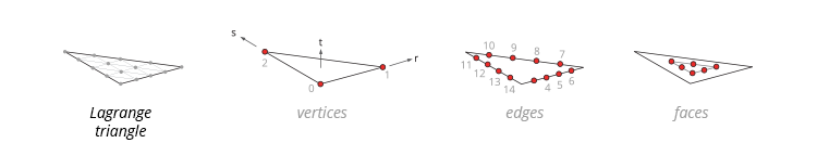
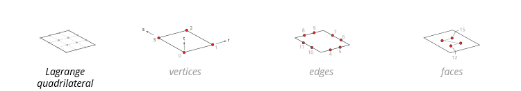
The number of points in a Lagrange cell determines the order over which they are iterated relative to the parametric coordinate system of the cell. The first points that are reported are vertices. They appear in the same order in which they would appear in linear cells. Mid-edge points are reported next. They are reported in sequence. For two- and three-dimensional (3D) cells, the following set of points to be reported are face points. Finally, 3D cells report points interior to their volume.

For simplicial shapes such as triangles, edge points are reported in a counterclockwise order. This order matches the order in which the points would appear in standard representations. Face points are reported next. They are reported as the points of a lower-degree Lagrange triangle. Vertices on this lower-degree triangle are reported first, followed by edge points and then face points, as described above. For higher orders, the process of reporting face points repeats until no points remain.
Like triangles, tetrahedra are simplicial shapes. Therefore, tetrahedral points are reported using the same method of recursion that is used to report triangular points.
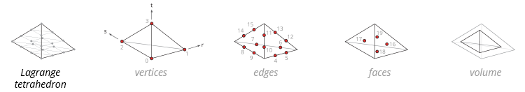
For higher orders, the process of reporting face points repeats per triangular face. To report volume points, the outer shell of vertices, edge points and face points is removed. What remains is a lower-order Lagrange tetrahedron. Vertices on this inner tetrahedron are reported first, followed by edge points and face points. The process of removing shells repeats until no points remain. In this manner, reporting points is like peeling an onion.
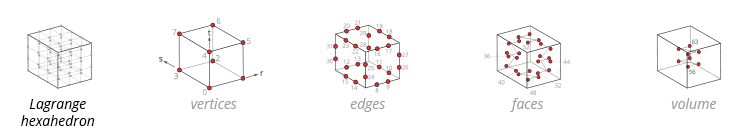
For prismatic shapes such as curves, quadrilaterals and hexahedra, points are reported on the boundaries first – from corners, to edges, to faces – followed by the interior, from the lowest r, s or t parameter to the highest. When reporting boundaries, the same pattern as the interior is used, but with fewer parameter dimensions used. This matches the order used for VTK’s existing fixed-order cells.
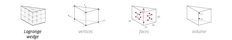
Wedges adopt the prismatic cell ordering with two exceptions: one for triangular faces and one for quadrilateral faces. On triangular faces, edge points are ordered counterclockwise. On quadrilateral faces, face points are reported in axis order. The axis that connects the first two points on each face can be traced from quadrilateral to quadrilateral on a path that proceeds counterclockwise around the triangular faces.
Example Code
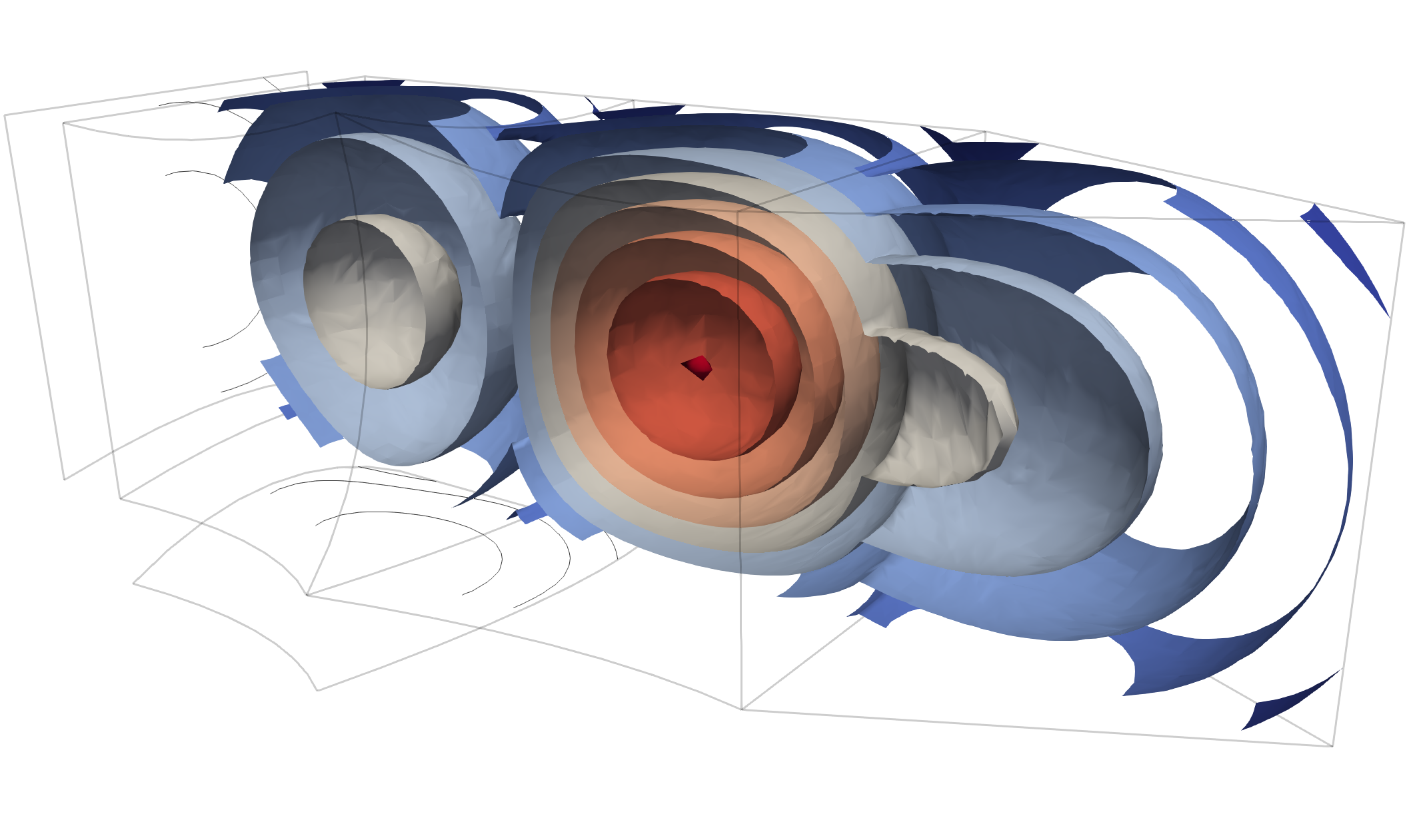
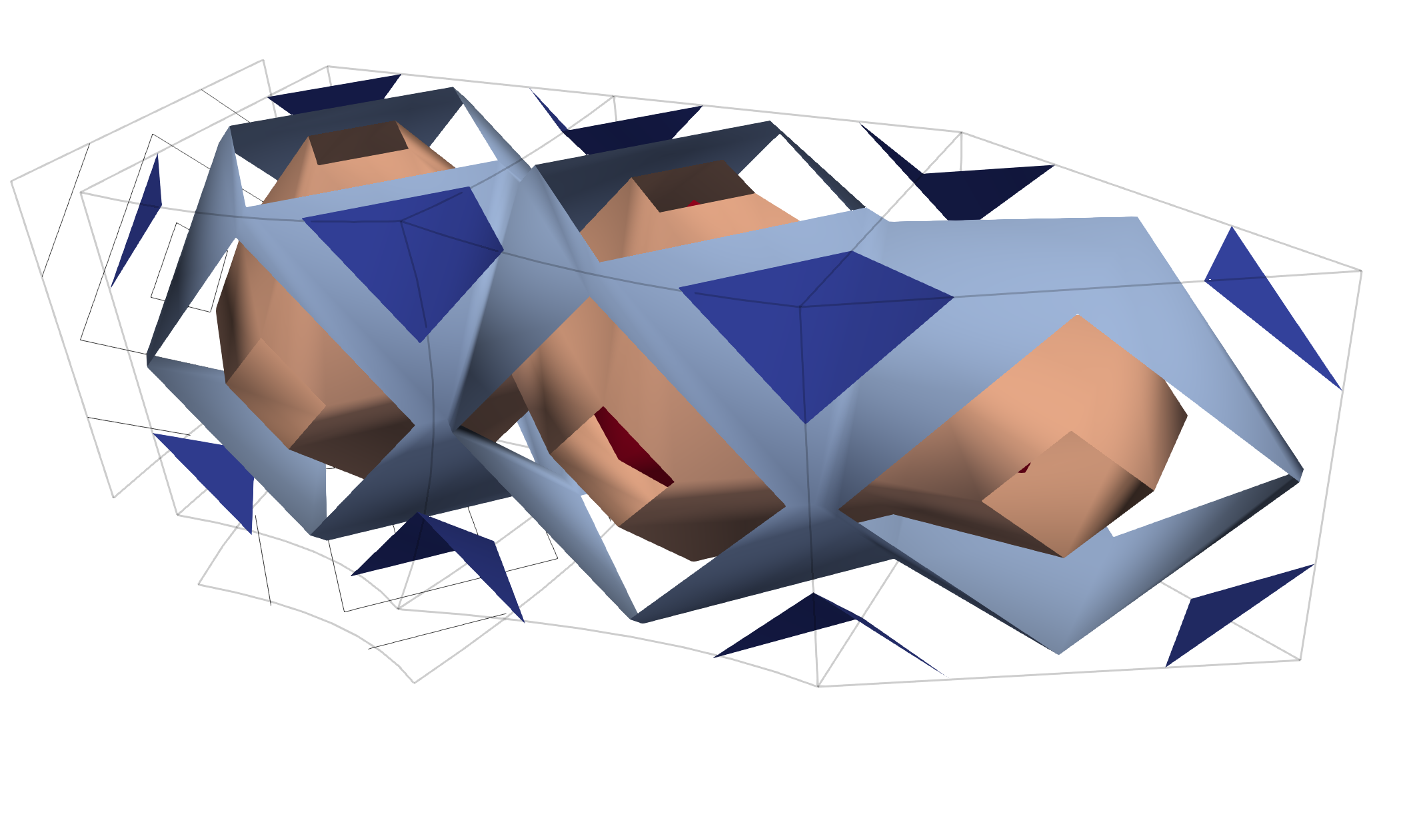
The pre-existing eXtensible Markup Language-based (XML-based) readers/writers in VTK have been extended to handle Lagrange cells. An example file is located on https://data.kitware.com in the Lagrange Cell Examples collection. While some elements in the example have a curved shape, every element has a curved (ellipsoidal) scalar function that is defined over each cell. This scalar function illustrates that higher-order cells can have interior minima, maxima and other critical points, unlike many linear cells.
The following Python code describes how to create individual cells and add them to an unstructured grid to make a Lagrange tetrahedron.
import math
import vtk

# Let’s make a sixth-order tetrahedron
order = 6
# The number of points for a sixth-order tetrahedron is
nPoints = (order + 1) * (order + 2) * (order + 3) / 6;

# Create a tetrahedron and set its number of points. Internally, Lagrange cells
 # compute their order according to the number of points they hold.
tet = vtk.vtkLagrangeTetra()
tet.GetPointIds().SetNumberOfIds(nPoints)
tet.GetPoints().SetNumberOfPoints(nPoints)
tet.Initialize()

point = [0.,0.,0.]
barycentricIndex = [0, 0, 0, 0]

# For each point in the tetrahedron...
for i in range(nPoints):
  # ...we set its id to be equal to its index in the internal point array.
  tet.GetPointIds().SetId(i, i)

  # We compute the barycentric index of the point...
  tet.ToBarycentricIndex(i, barycentricIndex)

  # ...and scale it to unity.
  for j in range(3):
      point[j] = float(barycentricIndex[j]) / order

  # A tetrahedron comprised of the above-defined points has straight
  # edges.
  tet.GetPoints().SetPoint(i, point[0], point[1], point[2])

# Add the tetrahedron to a cell array
tets = vtk.vtkCellArray()
tets.InsertNextCell(tet)

# Add the points and tetrahedron to an unstructured grid
uGrid =vtk.vtkUnstructuredGrid()
uGrid.SetPoints(tet.GetPoints())
uGrid.InsertNextCell(tet.GetCellType(), tet.GetPointIds())

# Visualize
mapper = vtk.vtkDataSetMapper()
mapper.SetInputData(uGrid)

actor = vtk.vtkActor()
actor.SetMapper(mapper)

renderer = vtk.vtkRenderer()
renderWindow = vtk.vtkRenderWindow()
renderWindow.AddRenderer(renderer)
renderWindowInteractor = vtk.vtkRenderWindowInteractor()
renderWindowInteractor.SetRenderWindow(renderWindow)

renderer.AddActor(actor)
renderer.SetBackground(.2, .3, .4)

renderWindow.Render()
renderWindowInteractor.Start()
Presently, the unstructured grid stores the X-Y-Z coordinate data, point field values and offsets for each point in data arrays. The overhead for this storage increases quickly with order. For hexahedra of order N along each axis, the overhead is (N + 1)3.
In the future, it may be possible to condense connectivity storage to a fixed size per cell shape. It may also be possible to specify order per axis rather than infer it from the number of points that define a cell. If order is explicitly specified, the following can be defined in memory: the offset to the first point and the order over which the points are iterated relative to the parametric coordinate system of the cell.
The VTK development team has already taken the first step toward these possibilities by keeping points for edges and faces together in Lagrange cells. After further steps are taken, the ability to relate points to a particular boundary will allow VTK to refer to the points with a single offset. This will allow VTK to significantly reduce its memory footprint.
Unit Tests
VTK offers unit tests for Lagrange cells. Some C++ unit tests are available in Common/DataModel/Testing/Cxx. LagrangeInterpolation.cxx, for example, evaluates the shape function that is common to tensor product shapes such as curves, quadrilaterals, hexahedra and wedges. Alternatively, TestLagrangeTetra.cxx, TestLagrangeTriangle.cxx and LagrangeHexahedron.cxx contain unit tests for inherited cell functions.
Python integration tests are located in Filters/Geometry/Testing/Python/LagrangeGeometricOperations.py.
These tests demonstrate how to read in new cells from an XML file, intersect the cells with lines, glyph the resulting points and run filters on the unstructured grid that contains the cells. One such filter is vtkUnstructuredGridGeometryFilter. It has been extended to demonstrate high-fidelity polynomial refinement. The technique renders representations that reveal the smooth nature of elements.
Adaptive Tessellation
To further reveal the true shape of elements, VTK performs adaptive tessellation. This technique is executed by vtkTessellatorFilter. The filter adaptively subdivides edges according to tolerances that are specified on the chord error and field value differences. The resulting isocontours are smoother than those produced with the default option. The reason why vtkTessellatorFilter is not the default option is because it is computationally expensive.
In addition to VTK, vtkTessellatorFilter can be used in ParaView. ParaView is a VTK-based open source software platform. As a result of recent changes, it now also supports Lagrange cells.
Acknowledgment
For funding the work on the Lagrange cells, the authors thank the Data Analysis and Assessment Center (DAAC) of the Department of Defense. Information on DAAC is available on https://daac.hpc.mil. DAAC has generously licensed the work so that others can benefit from it through the license for VTK. The license is detailed on https://www.vtk.org/licensing.
 Thomas J. Corona is a senior R&D engineer at Kitware. Among his interests are computational electromagnetics, mesh generation and high-performance computing.

David Thompson is a staff R&D engineer at Kitware. His interests include computational simulation and visualization, conceptual design, solid modeling and mechatronics.
There seems to be an issue with the indexing of the Lagrange hexahedron as shown in the picture. I tried writing a .vtu file by hand with the exact same indexing and visualizing it in ParaView and it did not show a correct hexahedron. Maybe you could correct the ordering of the indices.
Below you can find my vtu file for an order 3 Lagrange Hexahedron.
0 0 0
3 0 0
3 3 0
0 3 0
Hi Florian,
Instead of trying to debug your example (I am really overbooked right now), I will point you to the implementation of
vtkLagrangeHexahedron::PointIndexFromIJK(int i, int j, int k, const int* order); it should allow you to determine the connectivity that will work if there is an error in the figure. The last argument should be a 4-tuple holding(N, N, N, (N+1)*(N+1)*(N+1))whereNis the order of the element. Since your example’s point coordinates were integers starting at the origin, this function should let you plug in point coordinates and discover what connectivity entry that point corresponds to.Another technique for getting an example connectivity and coordinate array is to use ParaView. The “Unstructured Cell Types” source. Set the Cell Type to Lagrange Hexahedron, the Block Dimensions to (1,1,1), and the Order to whatever you want; the result will be a single Lagrange hexahedron of the specified order. You can save an ASCII XML file of the result and the connectivity will be easy to inspect with a text editor.
Meanwhile, I will file an issue to check the figure in the blog and Kitware source article. Sorry I do not have time for more than that right now, but I wanted to respond before things get too stale.
David
Hi Florian,
Instead of trying to debug your example (I am really overbooked right now), I will point you to the implementation of
vtkLagrangeHexahedron::PointIndexFromIJK(int i, int j, int k, const int* order); it should allow you to determine the connectivity that will work if there is an error in the figure. The last argument should be a 4-tuple holding (N, N, N, (N+1)(N+1)(N+1)) where N is the order of the element. Since your example’s point coordinates were integers starting at the origin, this function should let you plug in point coordinates and discover what connectivity entry that point corresponds to.Another technique for getting an example connectivity and coordinate array is to use ParaView. The “Unstructured Cell Types” source. Set the Cell Type to Lagrange Hexahedron, the Block Dimensions to (1,1,1), and the Order to whatever you want; the result will be a single Lagrange hexahedron of the specified order. You can save an ASCII XML file of the result and the connectivity will be easy to inspect with a text editor.
Meanwhile, I will file an issue to check the figure in the blog and Kitware source article. Sorry I do not have time for more than that right now, but I wanted to respond before things get too stale.
Hello,
Do you have any reference for the theory behind the Lagrange interpolation used here?
I’m trying to visualize the output from Nek5000, a spectral-element method solver that uses Gauss-Legendre-Lobatto (GLL) quadrature points inside the elements. I was able to create a vtk using LagrangeQuadrilaterals for 2D and LagrangeHexahedron for 3D. However, it looks like the interpolation is not the same as in Nek5000 and therefore the solutions are different when I sample along a line, for example. Nek5000 uses Nth-order Legendre polynomials which are orthogonal on the (N+1)^d GLL points, where d is the dimension of the problem.
Thanks,
Juan Diego
Hello Juan,
Here is a nice article describing the Lagrange shape functions for higher order quadrilaterals.
Sincerely,
T.J.
Hi Juan,
The one-dimensional Lagrange polynomials are described well here: https://en.wikipedia.org/wiki/Lagrange_polynomial . Extending them to 2 and 3 dimensions is covered in many books on finite element analysis. The one I used long ago was “Concepts and Applications of Finite Element Analysis” by Cook, Malkus, and Plesha (3rd ed., 1989), pp. 97-99. Another book, “Finite Element Analysis” by Szabo and Babuska (1991), ch. 6, p. 95ff. covers the Legendre polynomials. You are correct that the Legendre polynomials are a different basis. Note that for any two polynomial bases that span the same space (i.e., cover the same lattice of variable-exponent tuples across all terms of the basis), there is a linear relationship between their coefficients; you can translate from one basis to another by matrix multiplication. The condition number of the matrix will vary, and the Lagrange polynomial basis does not always produce well-conditioned matrices.
The quadrature points are slightly tangential to the polynomial basis; depending on your finite element solver, either the polynomial coefficients will be written out to specify the solution or the solution values at quadrature points (or both). You can usually obtain coefficients from the values at quadrature points and vice versa but this requires knowledge of the finite element formulation.
David
Hi David and T.J.,
Thank you both for your answers. This has been very helpful.
Juan Diego
Hi, in case anyone is struggling with the exact node ordering as I did, you can take a look at some python scripts I wrote for this purpose at this github repository.
node_ordering.pygenerates the point coordinates for a single Lagrange element of arbitrary type and order just like in the examples above, in the right ordering for VTK. Withsample_lagrange_element.pyyou can save this element to avtufile and view it e.g. in ParaView.The code Jens wrote was very helpful. Thank you very much. However as of Nov. 2023 when downloaded, for Hexahedron of higher polynomial degree there was a small bug.
def number_hexahedron(corner_verts, order):
“””Outputs the list of coordinates of a right-angled hexahedron of arbitrary order in the right ordering”””
# first: corner vertices
coords = np_array(corner_verts)
# second: edges
num_verts_on_edge = order – 1
edges = [(0,1), (1,2), (3,2), (0,3), (4,5), (5,6), (7,6), (4,7), (0,4), (1,5), (3,7), (2,6)]
The pattern for node distribution and edges and faces works great, but upon plotting the node numbering in Julia and the hexahedron it was slightly off. This is because the edge number was slightly off. The last line of code should be amended to
edges = [(0,1), (1,2), (3,2), (0,3), (4,5), (5,6), (7,6), (4,7), (0,4), (1,5), (2,6), (3,7)]
The edge ordering and corresponding nodes placed on edges now matches with the documentation provided above and that expected by paraview.
This fixed my bugs, and allowed me to easily go from general lagrange element ordering (for hexes) for arbitrary order.
Thanks again so much!
Hey Charles and Jens,
Thanks so much for your comments. I gave the Github repo a star and appreciate the work you put into making the script.
Jens — I notice in your code for the tetrahedron the following line:
faces = [(0,1,3), (2,3,1), (0,3,2), (0,2,1)] # x-z, top, y-z, x-y (CCW) TODO: not as in documentation, beware of future changes!!
I believe this is in fact the correct ordering of faces according to the documentation. Am I missing something?
Hi all,
This is updated in a fork, which should come back into Jens’ repo with an PR.
https://github.com/larsgeb/vtk-higher-order
Cheers,
Lars