This is a guest blog post from Martin Becker and Ulrich Heck, long time ParaView users. They work at DHCAE Tools GmbH, a German company focused on Computational Fluid Dynamics and Finite Element Analysis based on open source solver technology like OpenFOAM, CalculiX and ParaView.

Introduction

Spray simulations are a key tool in understanding the atomisation of molten metal with the help of gas jets. Such simulations combine complex multi-physics phenomena: ligament breakup, droplet formation, droplet–gas interaction, and ultimately solidification into particles. Post-processing these results in ParaView is crucial not only for scientific analysis, but also for communicating findings to broader audiences.

In this article, we demonstrate how different ParaView techniques can be applied to explore and visualise a transient OpenFOAM case of molten metal spray atomisation. From showing the full system context to highlighting droplet–jet interactions and producing high-quality animations, we aim to provide practical workflows that are both technically sound and visually compelling.

Eye Candy – Context Matters

To support the interpretation of the actual simulation results, it is often helpful to also display parts of the surrounding equipment. For non-CFD experts, the view inside the fluid domain can be difficult to interpret in isolation. Instead, the visible and tangible solids around the flow region provide intuitive context.

In our case of the metal nozzle and the annular nozzles, we therefore do not only show the “inlets” and “walls” of the CFD boundaries, but also larger portions of the real component – including inner and outer walls, suspension elements, and supply lines.

Since these areas on the “other side” of the flow domain are not required for the OpenFOAM simulation itself, the raw OpenFOAM boundary mesh is of limited use for this purpose. Instead, the STL input data that was originally used by snappyHexMesh is much better suited for visualisation. These STL files were exported directly from CAD as high-resolution triangulated surfaces. In addition, we sometimes export extra assemblies that are not required for the calculation but help to convey the function and geometry of the installation.

As a best practice, we keep a dedicated directory outside the OpenFOAM case, containing all STL files that are useful for visualisation. During post-processing with ParaView, these files can be loaded alongside the simulation results. Over the course of a project, this library can be enriched with further boundary representations – for example, specific OpenFOAM patches (inlets, outlets, faceZones, walls). These can easily be extracted (Filters → Alphabetical → Extract Blocks) , processed (with Slice, Clip etc), and finally exported from ParaView via File → Save Data → VTK Multi Block Files (*.vtm) for reuse.

The separate import of assemblies, boundaries, or patches makes it possible to apply targeted colouring (Solid Color), further improving clarity and allowing us to highlight specific components or surfaces of interest. STL files can be imported directly in ParaView (File → Open → *.stl or *.vtm), after which they appear in the Pipeline Browser ready for colouring. Besides applying colours, the Opacity can also be adjusted to create transparency effects. This makes it possible to indicate the position of components without obscuring the actual simulation results.

ParaView pipeline steps used in this view

• Geometry import
  • Load STL files (File → Open → *.stl or *.vtm)
  • Import assemblies or additional boundaries as needed
• Visual adjustments
  • Apply Solid Color to highlight components
  • Adjust Opacity for transparency effects
• OpenFOAM specific patches
  • Filters → Alphabetical → Extract Block with patches and faceZones of interest
• Optional
  • Export OpenFOAM patches as VTK (File → Save Data → *.vtm) for reuse

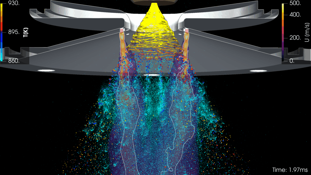
Figure 1: Overview of the setup with a sectional view through the ring nozzle. The hot molten metal is atomised and cooled by the surrounding gas jets. Temperature effects and jet structures are highlighted.

Introducing the Whole System

To guide the reader and viewer, it is often useful to start with an overview of the entire setup. Here we use the previously discussed STL files of the equipment components to illustrate the geometry and spatial arrangement. At the centre is the metal spray, coloured by the temperature distribution of the molten alloy. A black background enhances visibility, ensuring that even the smallest droplets and ligaments stand out clearly.

The second main component of the composition is the nozzle assembly with its support structure. The ring-shaped nozzle delivers the high-velocity inert gas that atomises and cools the molten metal. For the simulation itself, only the immediate nozzle outlet (a few millimetres in depth) is required, but for visualisation purposes the full ring nozzle with suspension is shown in metallic silver. A Clip filter cuts the assembly along its centre plane, exposing the spray core. The camera is positioned at a slightly upward angle, enabling the rear shape of the ring nozzle to be understood intuitively. An additional Slice filter through the nozzle centre provides a cut line, which is rendered as a fine silver tube (Filters → Alphabetical → Tube) to give the cross-section a stable and more massive appearance.

The nozzle function is further illustrated by the gas jets. The velocity field is clipped for |U| > 50 m/s and colour-mapped up to 500 m/s, revealing the shock-cell structures of the compressible jets. The jet cores are emphasised by an iso-contour at 50 m/s, generated with the Contour filter and displayed in white. This contour makes it easy to trace the jets visually, even through the ligaments and spray.

At the top edge of the scene, the outlet of the metal crucible (a hollow-cone nozzle) is shown in bronze colour. For now, the focus remains on the spray, with the nozzle’s internal air core only hinted at.

The overall composition is rounded out by legends for velocity and temperature ranges, making the key process parameters immediately accessible. The annotation of simulation time in milliseconds further highlights the time scales on which the dynamics unfold.

ParaView pipeline steps used in this view

• STL geometry (equipment)
  • Import STL files of nozzle assembly and crucible
  • Apply Clip filter (centre plane)
  • Apply Slice filter (centre plane)
  • Render slice line with Tube filter (silver colour)
• Spray (VOF field)
  • Colour by temperature field
  • Background set to black for maximum contrast
• Gas jets
  • Apply Calculator filter: mag(U)
  • Apply Clip filter: mag(U) > 50
  • Colour map: 50–500 m/s
  • Apply Contour filter at 50 m/s (white)
• Annotations
  • Add colour legends for velocity and temperature
  • Display simulation time in milliseconds

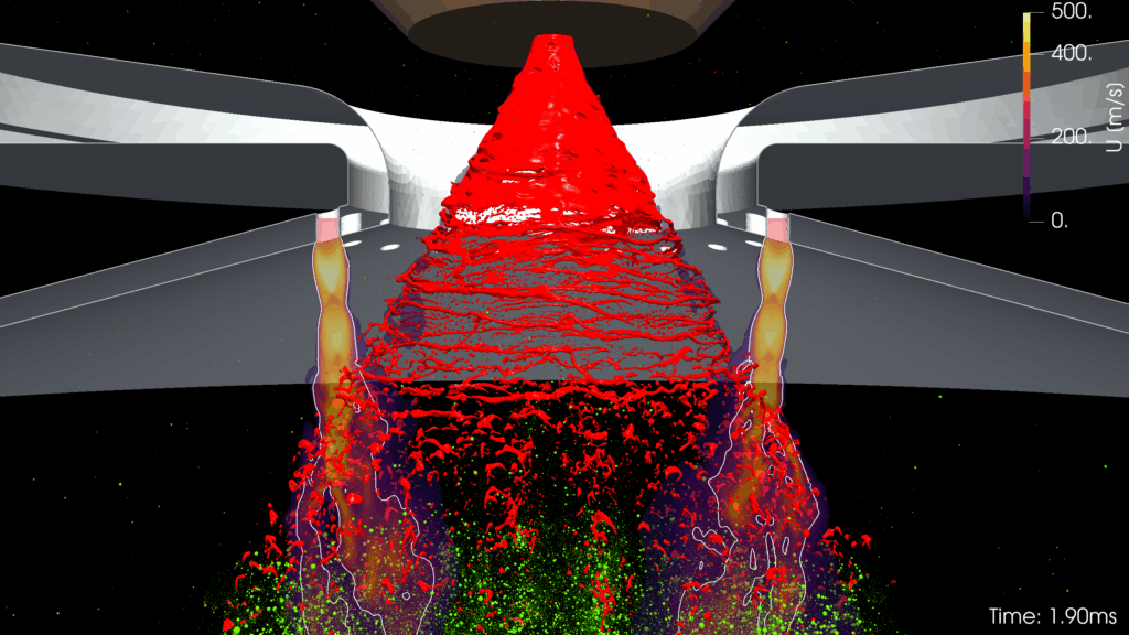
Figure 2: Red indicates the spray cone and the VOF-resolved ligaments. After conversion to Lagrangian particles, the droplets appear in green. Gas jets are displayed as transparent slices with highlighted velocity contours.

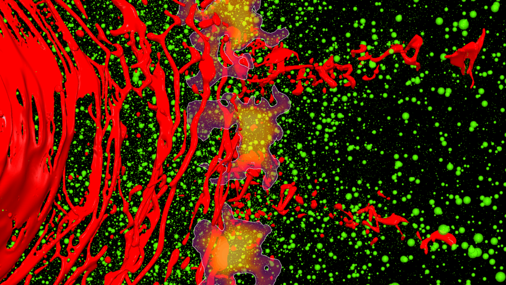
Figure 3: Top-down view showing how wide jet spacing allows red ligaments to pass through, while regions in contact with the jets are well atomised and form spherical droplets early.

Visualisation: Transition from Eulerian VOF to Lagrangian Modelling

A key element of our development is the efficient conversion of droplets formed during ligament breakup. Continuous ligaments are resolved with the Volume-of-Fluid (VOF) method, as are very large droplets or those that still pass through regions of strong interaction, such as droplet–droplet collisions or intense coupling with gas jets. Once these requirements for VOF modelling are no longer present – for example, when critical interaction zones are left and the droplets have become sufficiently spherical – they are converted on the fly into Lagrangian particles. Figure 2 focuses this transition zone of VOF to Lagrangian modelling. Transporting droplets in the Lagrangian framework is numerically much more efficient, and the mesh can be substantially coarsened under dynamic refinement.

To clearly visualise this conversion, we use contrasting colours: red for the VOF phase and green for spherical Lagrangian particles. Conversion is suppressed inside the gas jets to ensure that catastrophic ligament and droplet breakups are still resolved accurately. In these regions, the mesh resolution is still very fine; large Lagrangian particles would otherwise span more than a single cell, which cannot be represented consistently within the OpenFOAM methodology.

The figure 3 shows a top view of a side flank of the spray cone in, which is no longer fully continuous. Large ligaments and fragments enter the gas jets. Large ligaments and fragments enter the gas jets. The gas jets are represented in a slice view: a Calculator filter computes the velocity magnitude, which is then clipped at U > 50 m/s, leaving only the jet cores. These appear as cross-sections of the conical jets, coloured by velocity (bright yellow for nearly 400 m/s, dark violet for around 50 m/s). In addition, a Contour filter extracts the iso-surface at 50 m/s, resulting in a white line that highlights the jet shape. The slice planes are displayed semi-transparent so that the underlying ligaments and droplets remain visible.

The colouring of the molten metal (red ligaments vs. green converted droplets) clearly reveals the gaps between the gas jets. Large ligaments pass between the jets without being broken down to the target droplet sizes. Even though these ligaments eventually fragment into droplets, the resulting particles are too large – visible here as clusters of oversized green Lagrangian particles.

ParaView pipeline steps used in this view

• Ligaments and droplets
  • Colour by modelling phase (red = VOF, green = Lagrangian)
• Gas jets
  • Apply Calculator filter: mag(U)
  • Apply Clip filter: mag(U) > 50
  • Colour by velocity magnitude (50–400 m/s, violet → yellow)
  • Add Contour filter at 50 m/s (white line)
• Visual adjustments
  • Set jet slices to semi-transparent

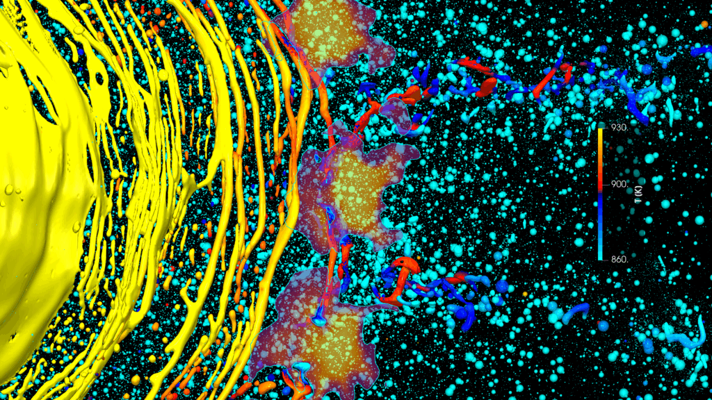
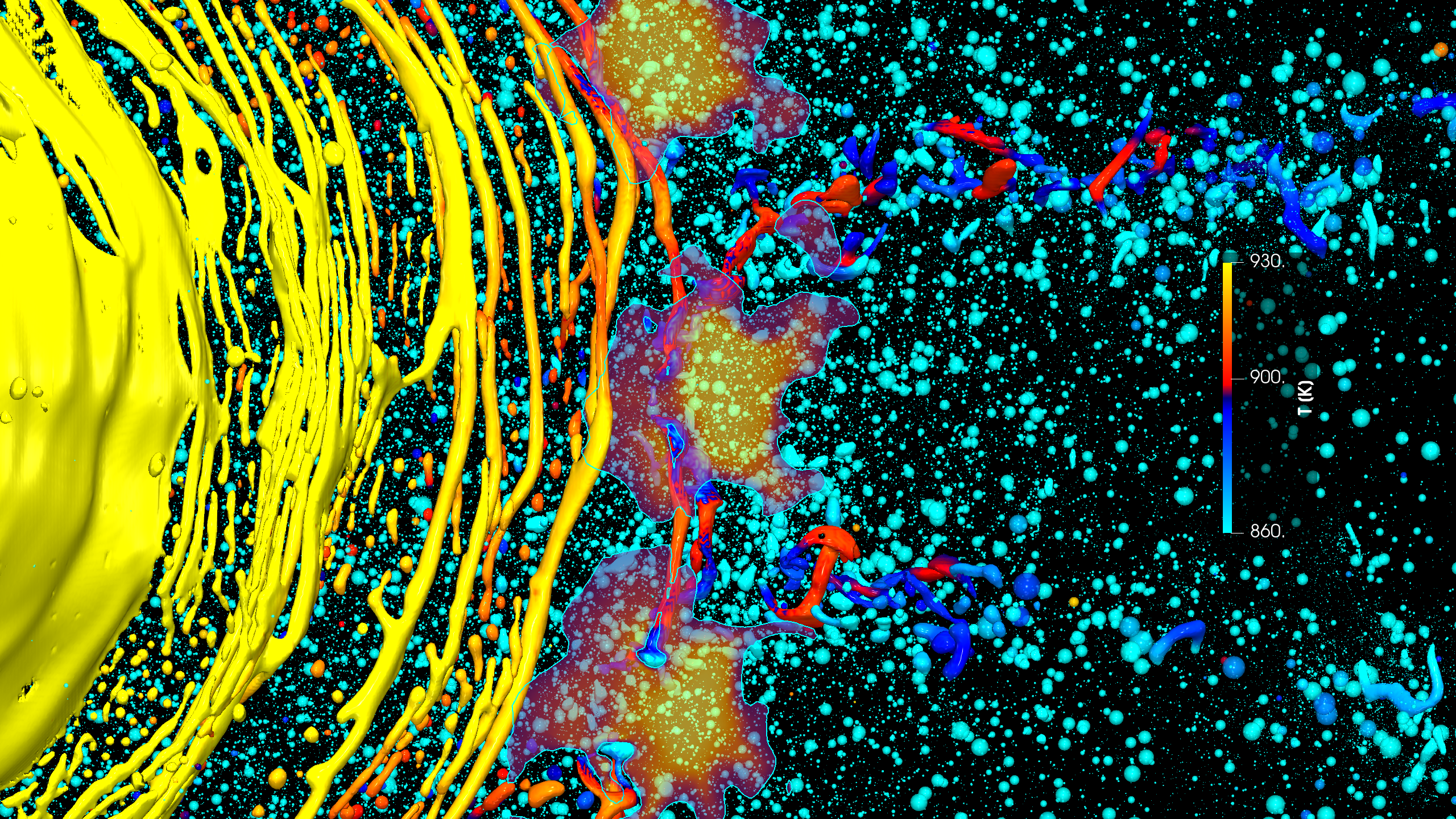
Figure 4: Temperature distribution in top view: yellow for fully liquid metal, dark blue to red for ligaments and droplets in the solidification range, and light blue for solidified particles.

A Slight Change of Focus

We now return to the same position at the outer flank of the spray cone and its interaction with the gas jets in figure 4. The jet cones are highlighted in the same way as before, but the focus is now on the metal temperature. The alloy is fully liquid above 930 K, completely solid below 860 K, and between these limits it passes through a solidification range. Lagrangian particles converted from droplets adopt the same temperature-based colour map as the ligaments and VOF droplets.

In most cases, VOF droplets are converted once they have become spherical and have left the jet interaction zone. In addition, the simulation automatically transforms VOF droplets below the solidification threshold into Lagrangian particles of equal mass, storing their last recorded sphericity. This allows us to assess both the final droplet form and the resulting powder quality.

The visualisation makes this behaviour easy to recognise: fully liquid metal appears in yellow as long as it exists as part of the spray cone or as large connected ligaments. When these structures come into contact with the cold gas jets, they undergo both fragmentation and rapid cooling. Droplets shown in light blue are fully solidified. Between the jet cones, however, larger ligaments and droplets are visible that are not completely broken down in the tested configuration. These regions also exhibit less cooling, leaving partially liquid ligaments passing through the jets without reaching the desired size or sphericity.

At the same time, some droplets are already transformed into Lagrangian particles due to their spherical shape, even though they may still be liquid or only partially solidified. Given the low relative velocity in the downstream flow, no further breakup of these round droplets is expected. Their ongoing cooling as Lagrangian particles, however, continues to be tracked.

In summary: yellow ligaments and VOF droplets upstream of the gas jets are favourable, and light-blue Lagrangian particles downstream are favourable. The critical issue lies with ligaments in the red to dark-blue solidification range that manage to slip between the jets. These can be clearly identified in the right-hand side of the visualisation.

ParaView pipeline steps used in this view

• Ligaments and droplets
  • Colour by temperature field (yellow = fully liquid, light blue = solid, red/dark blue = in solidification range)
  • Apply same colour map for both VOF and Lagrangian phases
• Gas jets
  • Same pipeline as previous section (Calculator → Clip → Contour, coloured by velocity)
• Annotations
  • Add legends for temperature and velocity
  • Display simulation time in milliseconds

Exporting High-Quality Animations

Creating a high-quality animation from a transient OpenFOAM case can be demanding in terms of time and storage. It is therefore important to minimise the number of iterations needed to reach the final result. One useful strategy is to decide on the final resolution early on. The target should be high enough to serve multiple purposes: detailed animations for exhibitions and presentations, but also scaled-down versions for social media or newsletters. While resolution and quality can always be reduced afterwards, improving a low-resolution export is nearly impossible. For this reason, we typically aim for a full resolution such as 2560 × 1440, which is a common YouTube video format.

During the setup in ParaView, however, working at such a resolution can be inconvenient – rendering slows down, and interface panels such as the Pipeline Browser or Colour Map Editor may become hidden. To keep the workflow efficient, ParaView offers Tools → Lock View Size Custom. By locking the view to 50% resolution (for example, 1280 × 720), the setup can be prepared quickly, while the aspect ratio is preserved. Test-exporting a single frame ensures the final sequence will look as intended. The full resolution is then selected only at the final export step (File → Save Animation).

For output format, we recommend exporting the sequence as individual PNG images. This lossless format avoids the compression artefacts that JPEG images can introduce, and the exported images can be reused for presentations, articles, or websites. The actual video animation is created in a second step. A widely used free tool for this purpose is ffmpeg, which combines the numbered image sequence into a high-quality video. A typical command looks like:

ffmpeg -framerate 25 -i “animation.%04d.png” -c:v libx264 myAnimation01.mp4

Complex processes are often best shown in multiple animations. In this case, we export several high-resolution sequences and later assemble them in a video-editing tool. This allows for adding explanatory text overlays, speeding up or slowing down sections, trimming, or merging into longer videos. The final export from the editing software also improves compatibility with platforms such as PowerPoint or online streaming, and offers control over file size through compression settings, formats, or reduced quality.

ParaView pipeline steps used in this workflow

• Resolution control
  • Use Tools → Lock View Size Custom (e.g. 1280×720 for preview, 2560×1440 for final export)
• Test export
  • Export single frame with File → Save Screenshot
• Final animation
  • Export sequence with File → Save Animation
  • Choose PNG as lossless output format
• Post-processing
  • Combine numbered PNGs into video with ffmpeg

Conclusion

ParaView provides a powerful toolbox for exploring multiphase spray simulations in depth. From contextualising results with CAD-based geometry, to distinguishing physical regimes through tailored colour maps, to producing publication-ready animations – each step enhances both scientific insight and communication.

The workflows presented here highlight practical strategies for handling complex datasets, while at the same time generating visuals that are engaging and accessible to broader audiences. Whether the aim is to analyse ligament breakup, droplet solidification, or to prepare a high-quality animation for presentations, ParaView enables researchers and engineers to efficiently bridge the gap between raw simulation data and compelling visual storytelling.

About DHCAE Tools

DHCAE Tools specialises in advanced spray simulations with OpenFOAM, focusing on atomisation, droplet cooling and solidification. Beyond model development, DHCAE Tools offers automation workflows and cloud-based SaaS solutions for scalable CFD.

Find out more:
– Website: www.dhcae-tools.com
– LinkedIn: DHCAE Tools on LinkedIn – https://www.linkedin.com/in/ulrich-heck-916359107
– YouTube: DHCAE Tools YouTube Channel – featuring the latest videos on spray simulations and post-processing https://youtube.com/playlist?list=PLC139PZ90-sRKdcWlWTI8RYBsPNcBG_av

– YouTube: DHCAE Tools – old and new examples of our post processing with ParaView https://www.youtube.com/@dhcaetoolsgmbh

About Kitware

Kitware delivers innovation to its customers. As a software research and development company, Kitware solves the world’s most complex scientific challenges using custom software solutions built on open source technology. In addition to custom software development, the company also offers technical support and training services to anyone using its open source tools. Since its founding in 1998, Kitware has developed a reputation for its unparalleled technical expertise and excellent customer service. The company is proud to be 100% employee-owned. For additional information, contact the experts at https://www.kitware.com/contact/.