AMR Contour and Interface support in VTK and ParaView
Introduction
Adaptive Mesh Refinement (AMR) is a popular method of numerical simulation used to adapt the accuracy of the simulation, which produces volumes of data of different levels of detail.
While this can be achieved using an unstructured grid, using a dedicated data model is preferred as it improves computation speed and memory usage.
Support for such data was added in VTK data model a long time ago with success although with a small adoption rate by the community and was recently deeply reworked as outlined in this blog.
In essence, an AMR dataset is just a collection of regular grids of different sizes and refinements, organized by levels, each more refined than the previous.
It comes in two flavors, OverlappingAMR and NonOverlappingAMR.
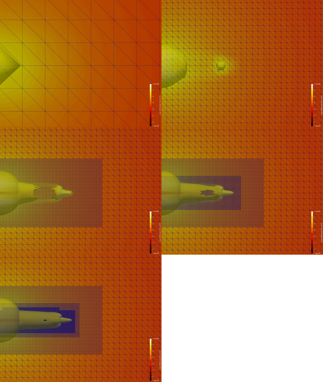

OverlappingAMR, as its name indicates, contains grids that overlap each other, with each level covering the whole domain. NonOverlapping, on the contrary, contains grids without any kind of overlap which is made for a more intricate grid organization at the higher levels.
OverlappingAMR is usually more efficient at the cost of some data duplication in the coarser levels, which we will focus on in this blog.
The contouring issue
Having different levels of refinement means that there are interfaces where, in essence, we have T cells.
A T cells, usually looks like that:
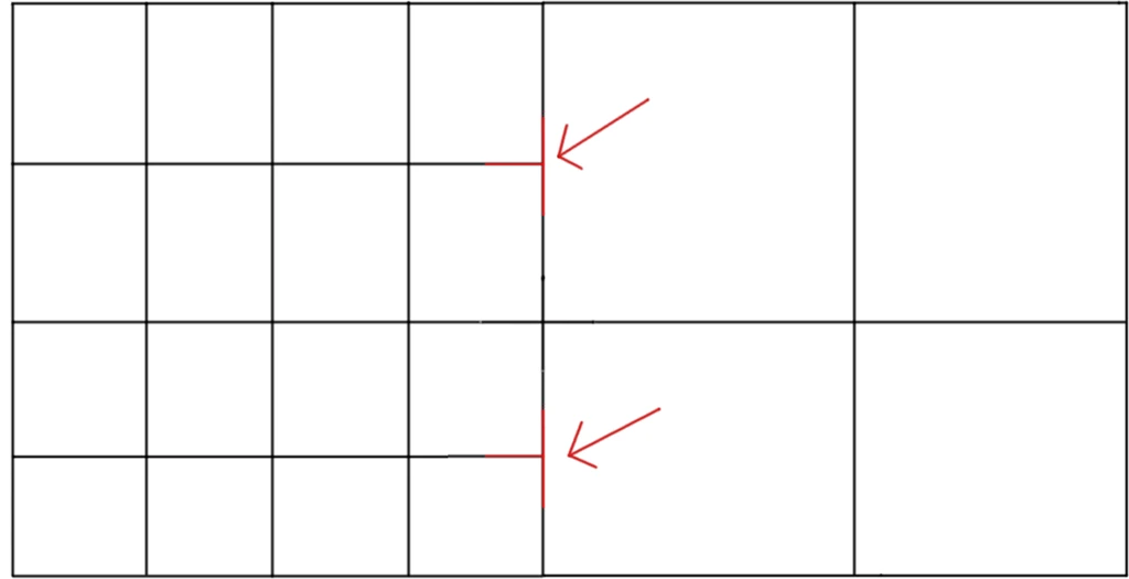
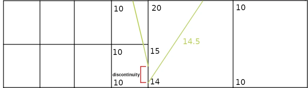
For many algorithms, a T cell acts as a discontinuity where the interpolation breaks from one cell to another. Indeed, both “central” points are only present in cells on the left side and not on the right.
In the specific case of the contour algorithm, where we generate isosurfaces (isolines in 2D) based on values interpolation, the result looks like this:
The solution is obviously to generate a proper interface in order to make this T cells disappear, generating new points and cells on the fly before running the contour:
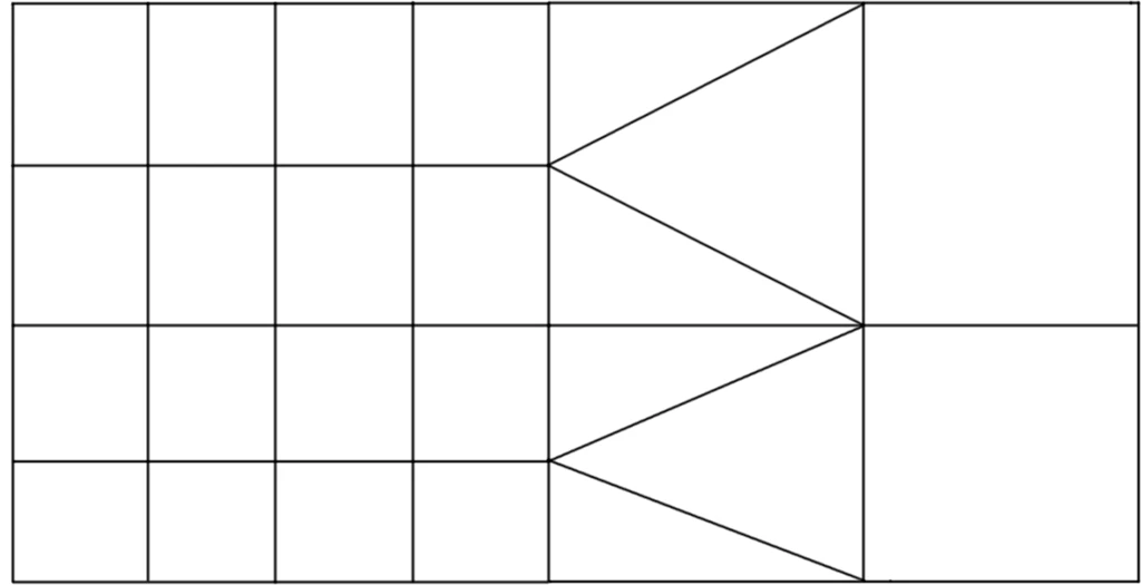
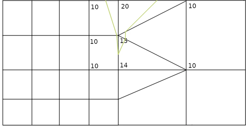
While this problem is generic of any kind of T cell, the particularity of AMR is that we know where those T cells are and where we should generate an interface, and all the cells we are dealing with are voxels, so this is a pretty fixable situation
Generating the interface
The illustrations above are in 2D and the resulting continuous interface is quite easy to visualize, but in 3D, the problem becomes a bit more complex. Here is how we do it.
The general idea of the algorithm is as follows:
The input is an overlapping AMR (aka a data object tree of cartesian grids).
The output is a partitioned dataset containing cartesian grids and unstructured grid.
For each block of the AMR:
- Identify each interface cells, hide them all in the block and add the block to the output
- Using all interface cells, construct on edges maps containing the points for the rough grid and points from the refined grid within the edge
- On each interface cells, construct a proper continuous interface using the edge map while interpolating data on the created points
- Add the interface cells as unstructured grid to the output
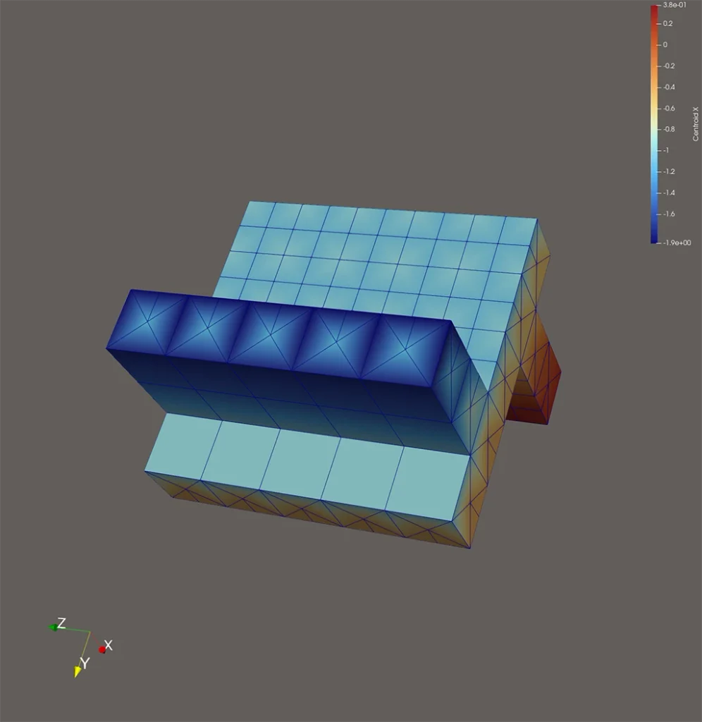
Considering that we work block by block, there will be an interface for each block, which will be generated where it “touches” a block of higher refinement. It also means that if there are edges that are part of more than two blocks of different refinement levels, the resulting interface may not be fully continuous. When tested on real cases, this case happened rarely and the resulting interface was always continuous anyway.
Interface cell identification
Identifying the interface cells is pretty easy, it is merely a matter of iterating over each point of each cell in the block and checking if this point is present in the overall AMR in a block of higher refinement. This is the most expensive part of the algorithm. If it is, the cell is part of the interface. The information about the point is stored for the next step as well.
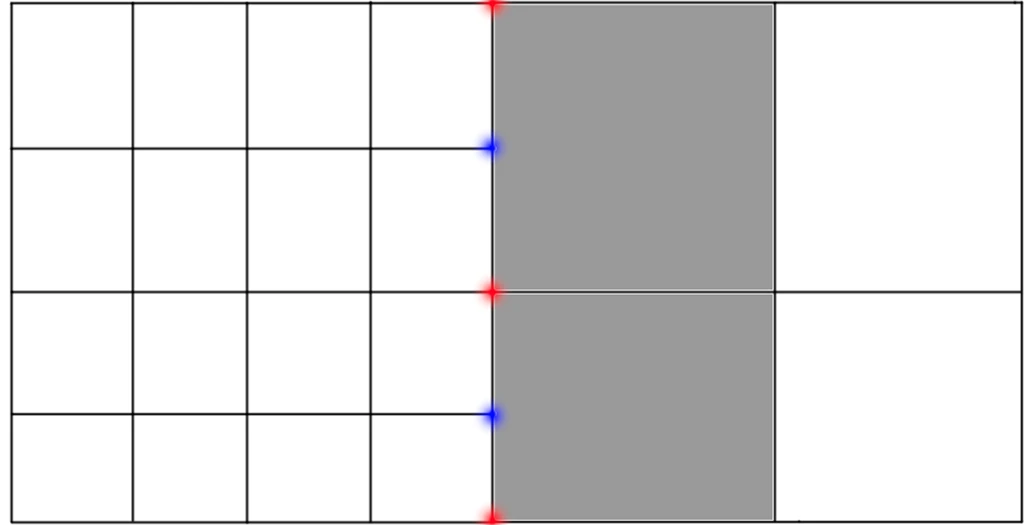
Edges iteration acceleration map
In order to reconstruct the interface, we need to know exactly which edges are refined and the location of the refined points on the edge. Since this will be used a lot by many different cells, finding the points on the refined edge only once is critical for performance.
In order to find them, it is needed to iterate over all points of all edges of all cells in the interface.
In our implementation this is done during interface cell identification.
An interface edge is an edge where both points are refined, and the center point of the edge is also in a refined block.
Once an edge has been identified as refined, the intermediary points must be recovered from the AMR. In order to do that, first the refined block is recovered, then the “WalkAxis” is computed, in order to know in which direction the edge is, X, Y or Z.
Using the direction, the edge can be walked on the refined block moving from one refined edge to the next. It is critical that the order of the edge points are kept.
It can happen that the edge is refined over multiple refined grids, in the case “contact” points are identified in order to know when to switch from one grid to another.
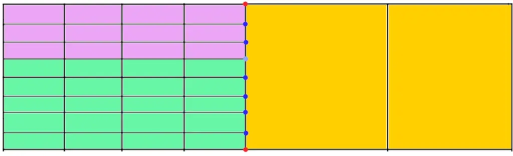
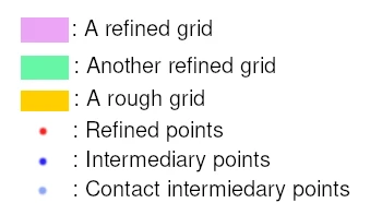
The result is a map of pairs of non-refined points to refined points that can later be used to reconstruct the interface.
Interface construction
To construct the interface, first the point data and cell data are initialized to contain the same structure as the grid, and a merging locator is also initialized as it will be used to create the interface unstructured grid, cell structures are also initialized.
Then we iterate on each voxel of the grid that has been flagged as part of the interface.
First we add the center of the voxel to the interface, as it will always be needed.
Then we iterate on each face of the voxel, recover each edge and center and identify one of three cases, either the face is a refined face, a non-refined face, or an interface face.
To identify the case, we simply count the number of refined points on the face, 4 (and center) is refined, 0 is non-refined and anything else is interface.
The non-refined case is trivial, we can just create a simple pyramid with the face as the base and the center as the top.
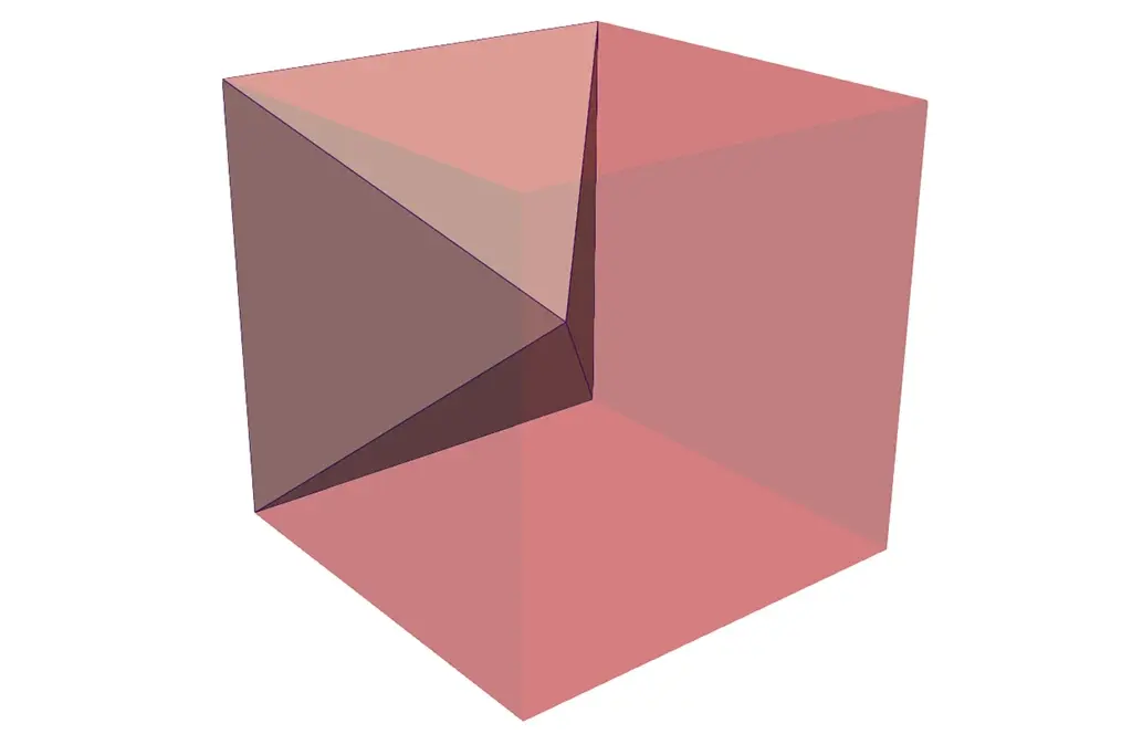
The refined case is a bit more complex, we must create many pyramids where the base is a square of refined points and the top is the center. Those refined points have to be recovered in the refined grids as they are not on the edges. Contact points are also critical to move from one grid to another while moving along the edges.
First the face must be cut into subfaces, where a subface is fully contained in a single refined grid, to do that we use the contact points on edges and are able to find the “opposite” point which is not on any edge. On most case each face contains a single subface which is itself, but it can be more complex than that.
Then we generate pyramids on the subface, one pyramid by refined voxels.
In order to do that we just iterate on both edges and create pyramids as we go using the subface points.
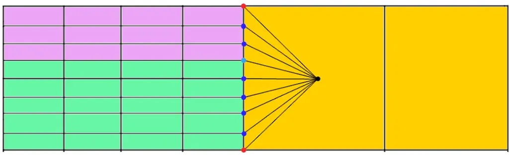
In black, the voxel center.
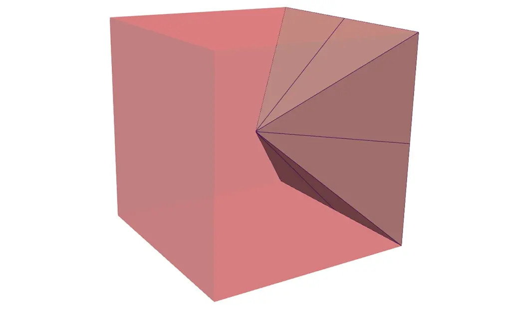
Finally the interface case requires us to fill up the spaces between refined faces and non-refined faces, which we do using tetrahedrons.
We check each edge of the face to see if it is refined or not.
If the edge is not refined, then we just create a tetrahedron using the edge, the face center and the voxel center. If the edge is refined, then we create tetrahedrons from each of the refined edge sections, the face center and the voxel center. This create a perfect paving between the single pyramid of non-refined faces and the multiple pyramids of the refined faces.
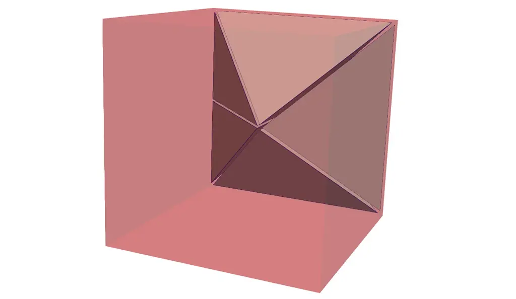
All the voxels are replaced by an interface the same way, resulting in coherency over the whole overlapping AMR.
Data Recovery and Interpolation
While creating the interface as described above, we are constructing an unstructured grid containing many points and cells, from the input overlapping AMR.
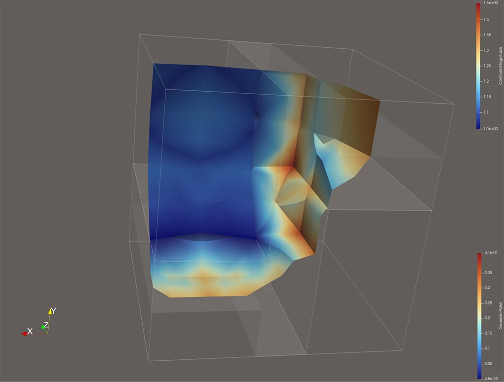
In order to be able to compute anything on the resulting output, we need to keep the point data and cell data around, however figure out the right values is not as trivial as it looks like.
For cell data, it is pretty simple, we just recover the cell data from the Overlapping AMR grid containing the unstructured cells and copy it.
For point data, it is more complex, there are two possibilities, either the point is present in the input grid, or it is a new point we created.
For points present in the grid, we must recover the data from the most refined grid available, in most cases we know which it is but in some cases it is required to copy the data multiple times until the most refined grid is reached.
For new points, interpolating is required. It concerns face center and voxel center.
For face center, we use all the existing points in the face and compute a simple shepherd interpolation.
For voxel center, we recover all points that were ever added for the paving, including the face centers and compute a simple shepherd interpolation.
The results can sometimes look a bit jaded when contouring from a very rough grid to a refined grid but it is enough for the purpose of generating a continuous interface.
Output construction
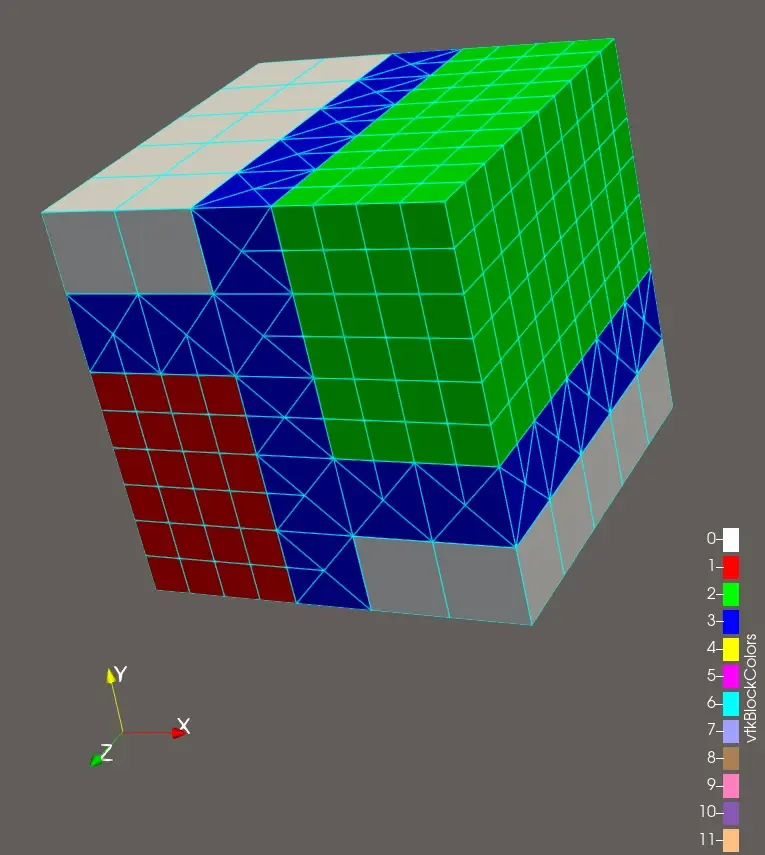
Reconstructing the output is quite trivial once we have the interface.
We just create a partitioned dataset containing the refined grids with the interface blanked out, and each of the unstructured grid interfaces for each refinement level.
Contour
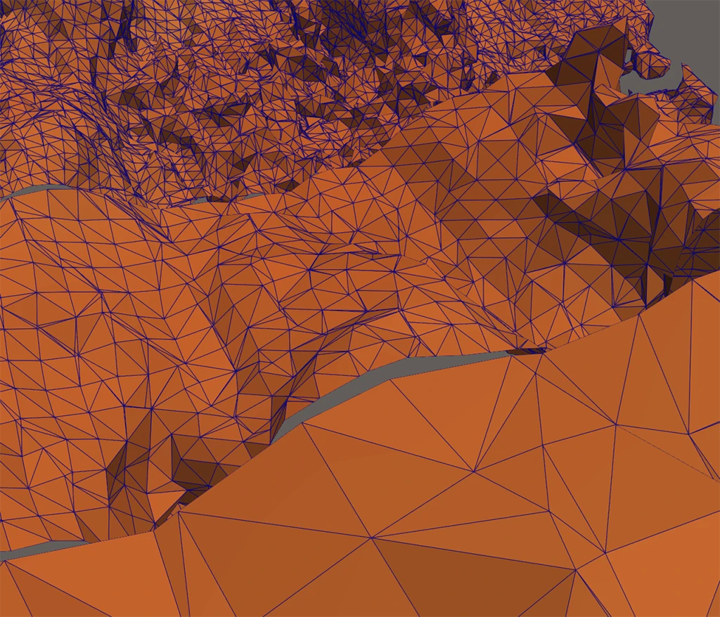
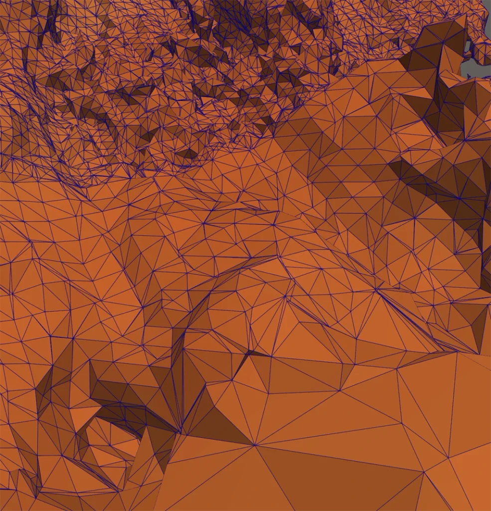
With the interface computed, computing the contour is pretty straightforward, we just run the standard contour filter on the whole partitioned dataset output while taking care of keeping the interface filter around to keep the benefit of the interface being already computed if only the contour value is changed when making multiple contour computation.
The has been integrated in ParaView and is available in ParaView nightly and will be available in ParaView v6.3.0
Perspectives
Distributed computation:
As of writing this, VTK does not support distributed AMR very well, so distributed AMR was not considered in the testing of this filter, however we are confident that it should work with minimal changes, and this is definitely something to address once distributed AMR is fully functional.
Other interpolation types:
While shepherd interpolation is enough in our case, it may be possible to use other kinds of interpolations to get better results.
Performance:
Most of the time is spent looking for which grid contains which points (vtkOverlappingAMR::FindGrid), which is already a call we try to reduce as much as possible thanks to the acceleration structure. So investigating how to make this call faster may be a possible performance improvement.
Acknowledgments
This work was funded by CEA, DAM, DIF, F-91297 Arpajon, France

Thanks for Jean Favre, CSCS and Håkon Strandenes, KMTurbulenz for providing test data.