Deep-learning surrogate models in ParaView: Viewing inference results and monitoring the training process in real time with Catalyst.
This article describes two recent developments concerning the integration of Deep-learning techniques in ParaView. First, ParaView has been adapted to visualize the results produced by a deep-learning-based surrogate model in real time. Next, Catalyst has been used to monitor the training process of this model.
Context
A surrogate model (of a numerical simulation) approximates a solver’s outputs with a low computational cost. Solvers of partial differential equations, for instance those based on finite elements methods, often require long runs. Thus, they are not well-suited for real-time applications. EDF Lab, which is the R&D department of one of the largest electric utility companies in Europe, is investigating the use of Deep-Learning to construct surrogate models. EDF engineers regularly run Computational Fluid Dynamics (CFD) simulations for systems such as windmills, steam generators, or turbines. These simulations produce large data sizes and take long computation times. They are consequently not useful for a variety of important applications, such as digital twins.
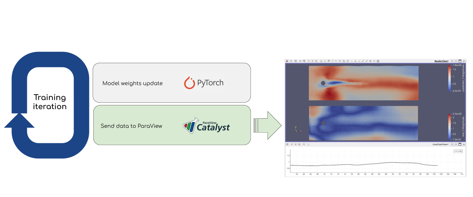
In this work, ParaView has first been adapted to visualize the results produced by a deep neural network in real time (the surrogate model). On a second step, Catalyst has been used to monitor the training process of the deep surrogate model. These developments have been validated on a use case representing Karman Vortex Street; where a fluid (entering with an imposed velocity on the left of a rectangular domain) flows towards a cylindrical obstacle and a set of vortices forms behind it. An ensemble of simulations was performed by EDF’s CFD solver Code_Saturne. Each member of the ensemble corresponds to a different imposed input velocity.

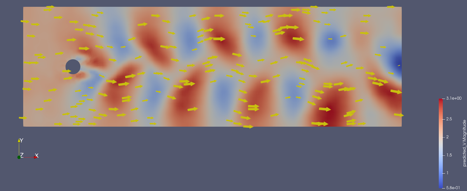
The deep neural network used to predict the results of these simulations was built using the Pytorch framework. It takes two parameters as input: the imposed velocity of the fluid and the time of the simulation. This surrogate then outputs a discretized velocity vector field. A depiction of this model is shown above. It is important to note that the mesh provided to study this problem is irregular, and presents finer cells around the obstacle. This irregular structure is taken into account by the neural network, which uses spline-based convolutions layers described in (2), and is designed to take into account the geometric structure of the problem. The figure below shows an example of an inference result visualized in ParaView, where a velocity vector is associated to each cell.
A ParaView Python plugin was developed for this project. Indeed, ParaView offers a thorough interface that allows the user to customize the pipeline with plugins which can be completely written in Python. This enables the merge of ParaView’s scientific visualization capabilities with the robustness of Python machine learning frameworks such as Pytorch, TensorFlow, Sci-Kit Learn, or Keras for the implementation of the model.
Running inferences with CUDA
We developed a ParaView filter to run inferences flexibly and directly inside of ParaView. It takes the mesh as input and predicts the resulting fluid velocity at each cell for the chosen (velocity, time) parameters by loading the pre-trained Pytorch model. As running an inference on this model uses CUDA, the different timesteps of the animation can be generated in real time.
The video below shows the results of the inference filter, once the turbulent flow is well established.
Monitoring the training process
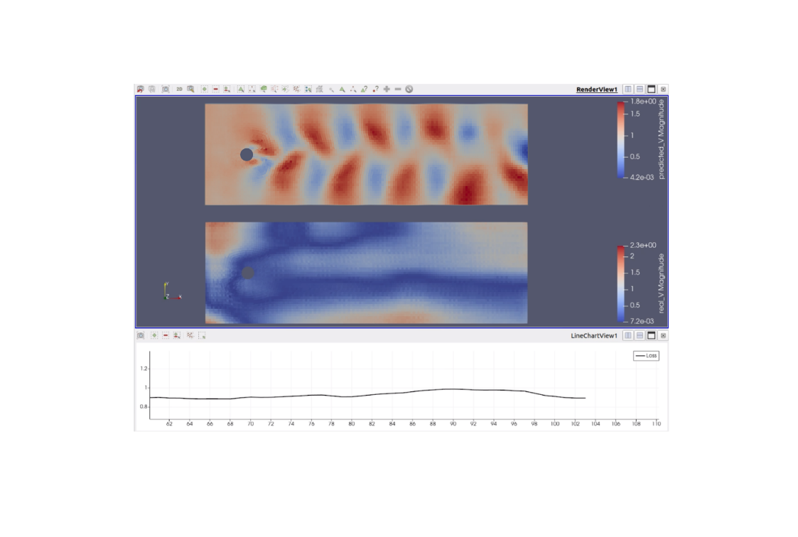
ParaView Catalyst is an in situ library that allows analysis on data located in the memory instead of reading it from the disk. This is useful for generating frames in real time while the simulation – in this case the training – is running in the background. The frames generated can be sent to a remote ParaView server which allows real-time visualization of the results with the ParaView Desktop application, or alternatively, can be saved on disk.
All of these features are available as soon as you adapt your code to run alongside ParaView Catalyst. This requires doing the following :
- Adding three different Catalyst API function calls to the main simulation code (initialize, coprocess and finalize)
- Creating an adaptor (or coprocessor) that will tell ParaView how to display the data you are passing to Catalyst
- Linking a ParaView Catalyst State script to describe the elements of the visualization pipeline.
More details about the implementation of a Catalyst pipeline can be found here. The video below shows how to visualize the training process in practice with ParaView Live.
To visualize how our model performs during training, and to identify which aspects of the simulation the model understands better and which aspects it struggles with, we chose an arbitrary fixed input (velocity, time). An inference is run each time the model weights are updated to check how well it performs on the chosen (velocity, time) tuple. On top of the inference results being displayed on the mesh, we can also access more generic data about the training process such as the loss or any other metric, and display it in a line chart view to see how it evolves over time. Any variable, array, or tensor can be passed to the Catalyst API as long as you have an idea of how to display it in ParaView.
Full training overview
The following video was created from the frames generated by Catalyst during training. It highlights the full training process of the model for a given (velocity, time) input.
The model quickly understands that a trail is forming behind the obstacle, and that everything around the trail has a lower velocity. Then, as the neural network keeps learning, it starts to understand that the trail is not uniform but consists of a set of alternating vortices. The vortices at the back (farther away from the obstacle) are the ones that are learned the quickest, while the ones at the front (close to the obstacle) seem tougher to grasp.
Conclusion
We were able to load a custom Python model with a ParaView plugin, run it with the desired input parameters inside of ParaView, and display its inference results on objects of the ParaView pipeline. This provides a flexible and convenient way to visualize the output of the model without having to generate the data externally. Furthermore, we followed and monitored the training process of a model in real time using ParaView Catalyst, allowing us to see how well the model performs after each training iteration, and helping us visualize the convergence of the prediction towards the desired results.
This work is a step towards making ParaView suitable for handling the full workflow of any machine learning project, providing its powerful visualization capabilities to help machine learning experts and data scientists have a deeper understanding of how their models work.
References
- Lucas Meyer, Louen Pottier, Alejandro Ribes, Bruno Raffin : Deep Surrogate for Direct Time Fluid Dynamics arXiv:2112.10296 [cs.LG]
- Matthias Fey, Jan Eric Lenssen, Frank Weichert, Heinrich Müller : SplineCNN: Fast Geometric Deep Learning with Continuous B-Spline Kernels arXiv:1711.08920
- AI in ParaView and LidarView: Point cloud Deep Learning frameworks integration with Python plugins
- Integrating Geometric Deep-Learning models into Paraview
Acknowledgements
This work is funded by an internal innovative effort of Kitware Europe, with a technical support of EDF R&D.