Explore large acoustic data with the Digital Signal Processing plugin in ParaView

In a previous blog post, we introduced the Digital Signal Processing (DSP) plugin in ParaView. If you want to learn how to use this plugin in a simple workflow, please skip to the how to use section. Stay tuned for our next blog about the implementation itself and benchmark results.

Although this plugin is functional, it was not complete nor performing at the expected performance, especially when it came to large datasets and distributed computing. These shortcomings have since been addressed, with a now complete workflow supporting large datasets and distributed computation. Of course, there is still room for improvements, especially in regards to missing features and filters that could be added in the future. Please contact us if you would like to contribute.

In the previous blog, we listed the available filters. This list has been expanded to include the following developments.

New Filters and Features

Temporal Multiplexing Filter

This filter is an optimized filter replacing the Plot Data Over Time filter for DSP analysis. It generates multidimensional arrays. It takes geometrical temporal data and extracts the data over time in arrays where the spatial dimension is a hidden dimension. See this [future] blog for more information about the multidimensional arrays and how it increases performace drastically.

Multi Dimension Browser

This is a simple filter to navigate through the hidden dimensions of the temporal multiplexer output. In essence, it lets you select a point of the geometry to work on, based on its index. When performing distributed computing, the pipeline browser uses global indexes for displaying single points at a time.

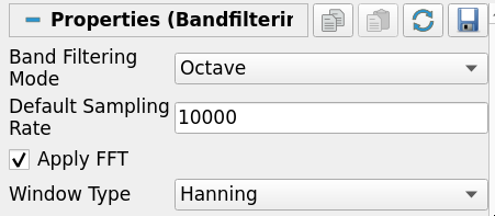
Band Filtering Filter

This filter performs a band filtering operation in frequency space. It takes as input a table with at least a column for a specific quantity and an optional time array. It’s possible to pick a custom band or choose between octave and third octave band. The output is a table with the mean of this quantity (in the original unit or in decibels) for each frequency defined in the frequency column (in Hz). 

Band filtering result on a microphone data

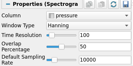
Image Chart View

This is a new type of view dedicated to displaying 2D image data in a chart context. It can be used with  the Spectrogram filter output. It comes with the same customization options as many other charts, such as axis properties, custom labels, etc. It also allows easier data inspection with axis annotations and tooltips.

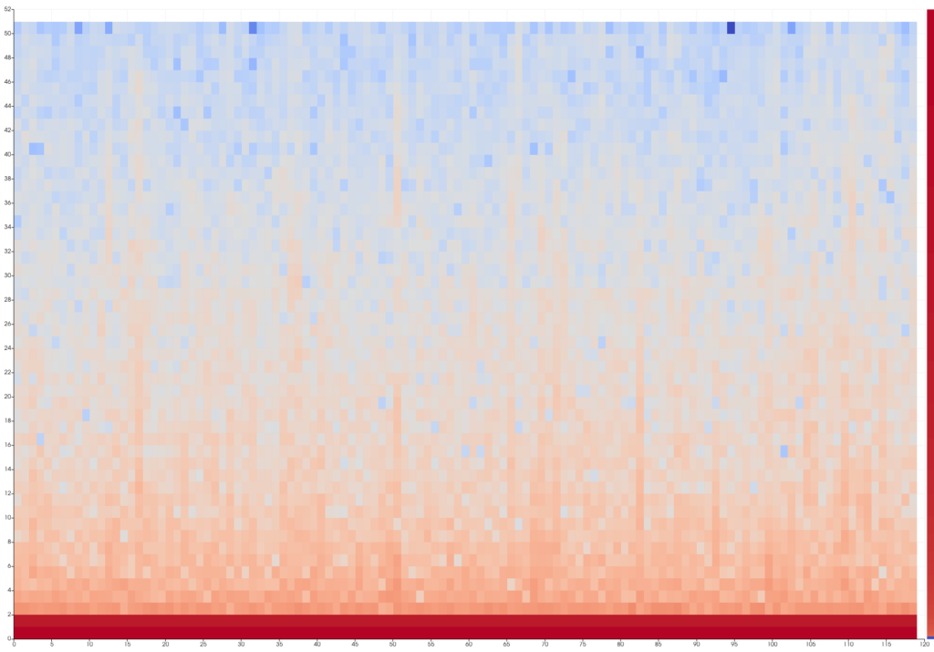
Spectrogram results shown in an ImageChartView with a lot scalar map

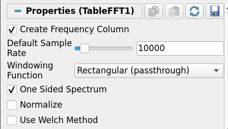
DSP Table FFT

This is a Fast Fourier Transform (FFT) filter dedicated to compute FFT on the output of the Temporal multiplexer. It has the same arguments as the usual Table FFT filter. Similarly to the Temporal Multiplexer, it outputs a table of multi dimensional arrays where the hidden dimension is still related to the spatial discretization and the tuple dimension represents the discretization of frequency space.

FFT result on a microphone using Welch method

Merge Reduce Tables

This is a simple filter to compute statistics and reductions across the spatial dimension of a table of multi dimensional arrays, such as the mean or the sum over columns.

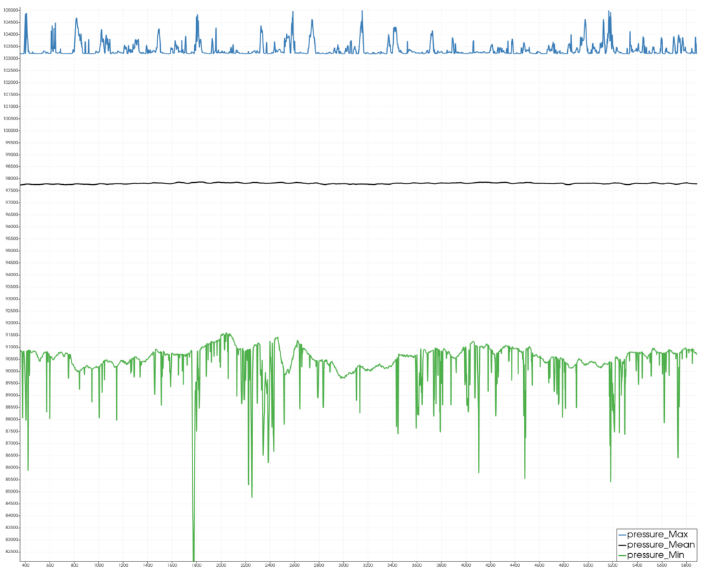
Pressure Min/Mean/Max on all microphones over time

How to use the Digital Signal Processing to do a basic acoustic analysis using ParaView

Let’s consider a typical use case : we have a geometry with acoustic data evolving over time that ParaView can open easily:

Acoustic simulation result of a landing gear, animated pressure over time

The first thing to do is to extract all data across space and time using the temporal multiplexer.

• Add a temporal multiplexer
• Select the array that is evolving over time, then press Apply.

The computation may take some time to compute and a consequential chunk of memory given that all time steps are being loaded.

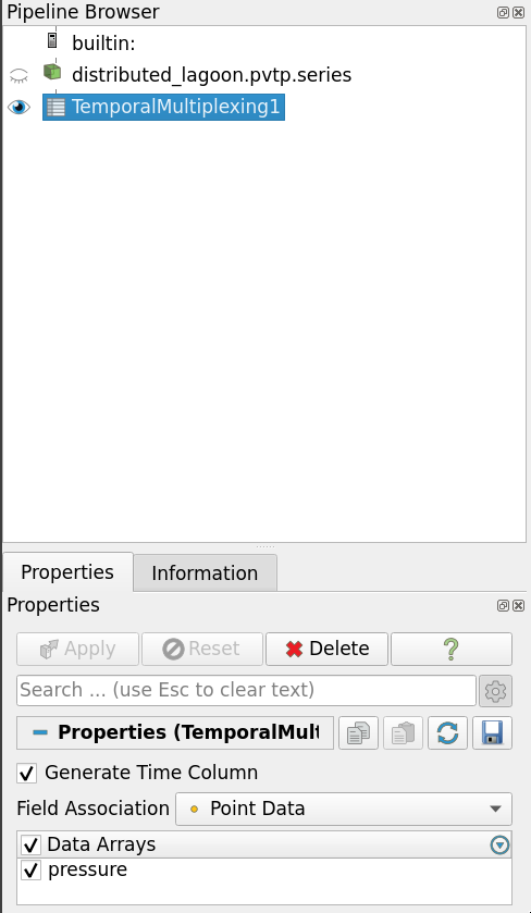
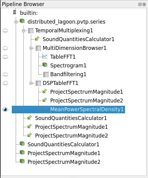
TemporalMultiplexer in the pipeline browser and its properties

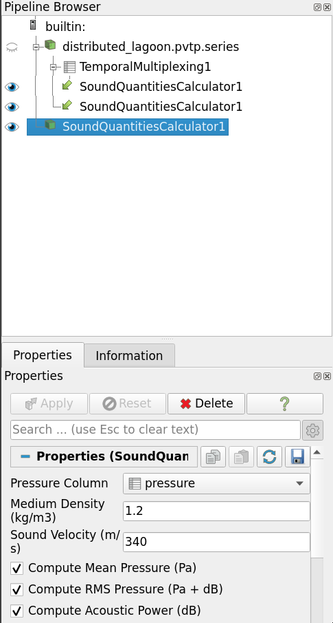
We can’t really exploit the output of the multiplexer directly but we can directly compute some metrics on it. Lets compute the Root Mean Square (RMS) using the Sound Quantities Filter. 

• Make sure the Temporal Multiplexer is still the active source
• Add the Sound Quantities Filter
• Select the original geometrical dataset as the destination mesh, select Pressure as the pressure column, press Apply
• Show the result in a render view, color by RMS

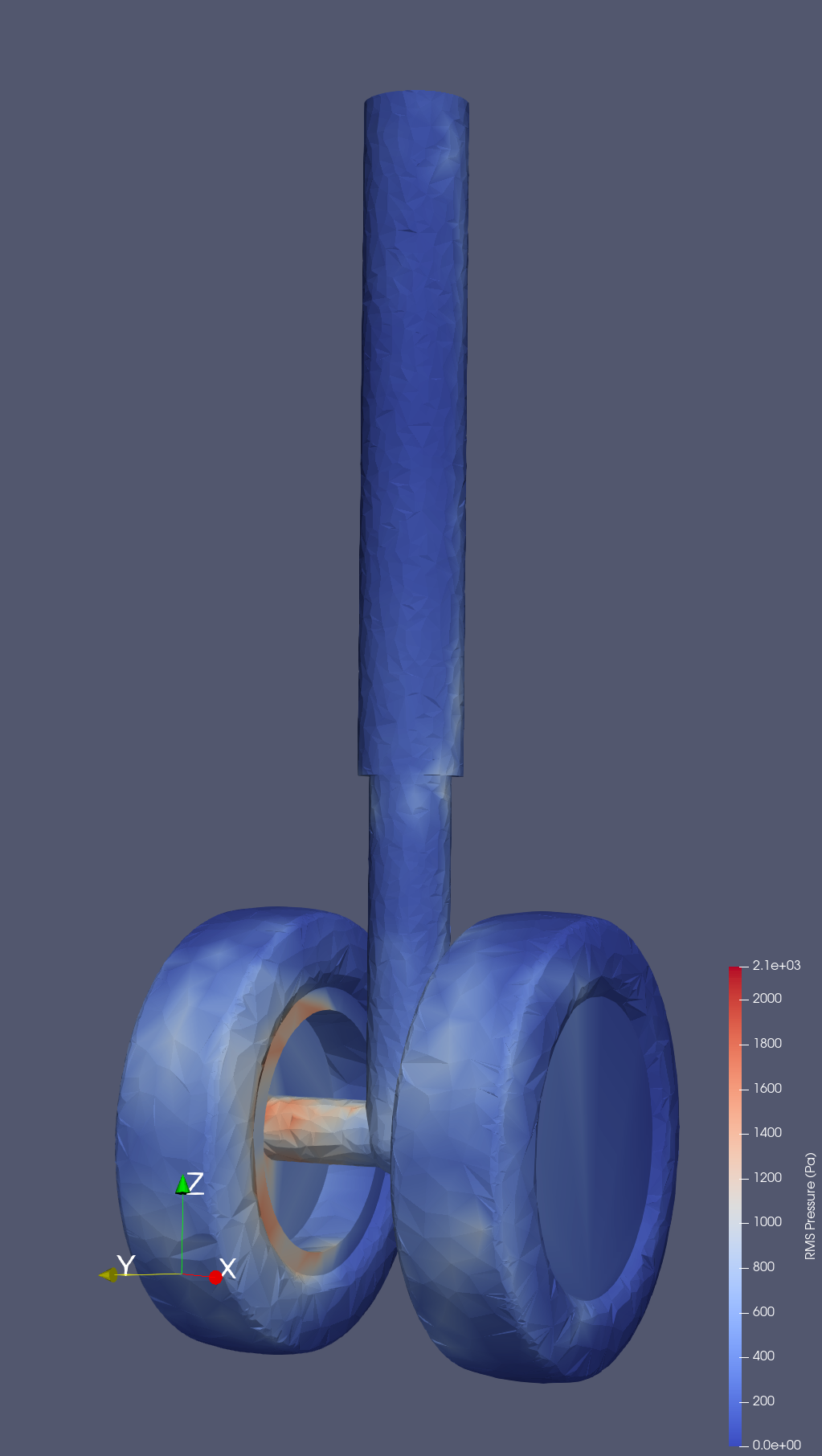
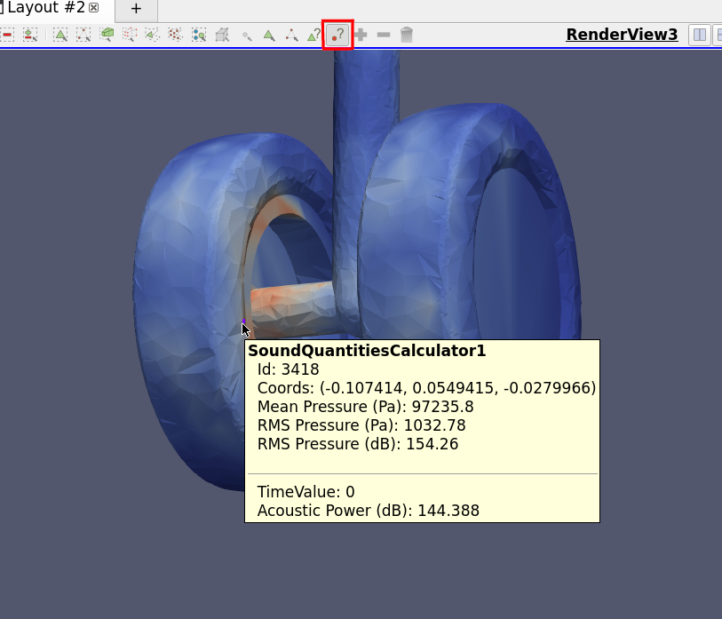
Visualization of the RMS (Root Mean Square) of an acoustic pressure over all timesteps

Now we are able to see more information, let’s try to focus on a specific point of the geometry. We can use `Hover points on` to select a point and find its id:

Using `Hover points on` to identify a point to inspect

Let’s extract data at this point and do some FFT, Spectrogram and BandFiltering computation

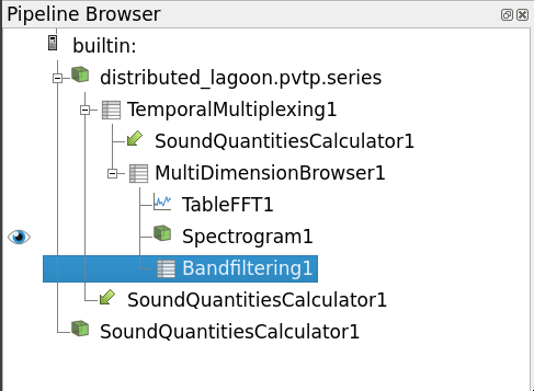
• Click on Temporal Multiplexing to make it active
• Add a Multi Dimension Browser, select the point id we chose earlier, Apply
• Add a Table FFT filter, choose the properties as needed, Apply
• Select the Multi Dimension Browser, add a Spectogram, select Pressure as column, change options as needed, Apply
• Select the Multi Dimension Browser, add a Band Filtering, change options as needed, Apply
• Create a new Layout, show the Spectrogram in an Image Chart View,
• Change the LUT to log
• Split the view, show the FFT in a LineChartView, set Left axis to log
• Split the view, show the Band Filter in a LineChartView, set Left axis to log

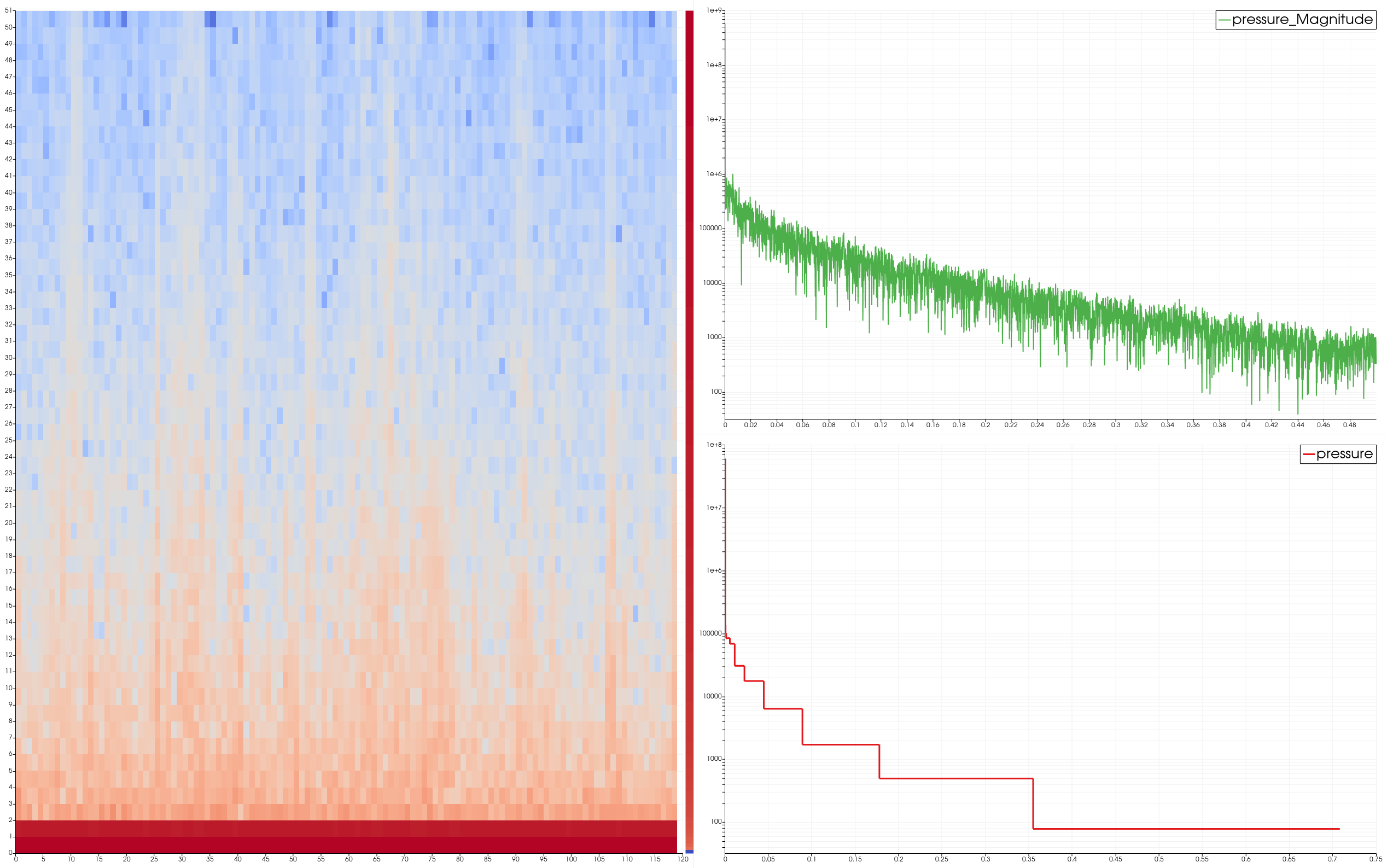
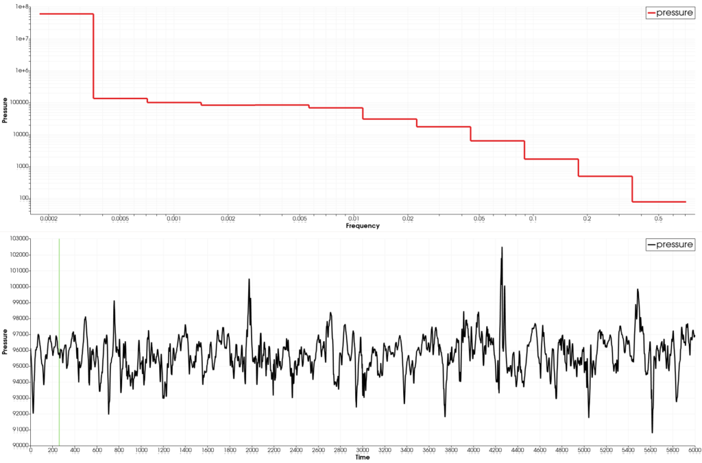
Multiview acoustic information of a single microphone

Now let’s compute the spectrum magnitude for different frequencies over the whole geometry. But first, we will need the FFT on the whole spatial domain and to use the dedicated filter

• Select the Temporal Multiplexer to make it active
• Add a DSP Table FFT, change options as needed, Apply
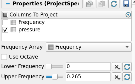
• Add a Project Spectrum Magnitude, select the geometry as destination mesh, set lower frequency bands, Apply
• Select the DSP Table FFT to make it active
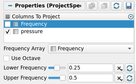
• Add a Project Spectrum Magnitude, select the geometry as destination mesh, set higher frequency bands, Apply
• Create a new layout, split in two render view, show each PSM in each view with a Camera link and separated color maps

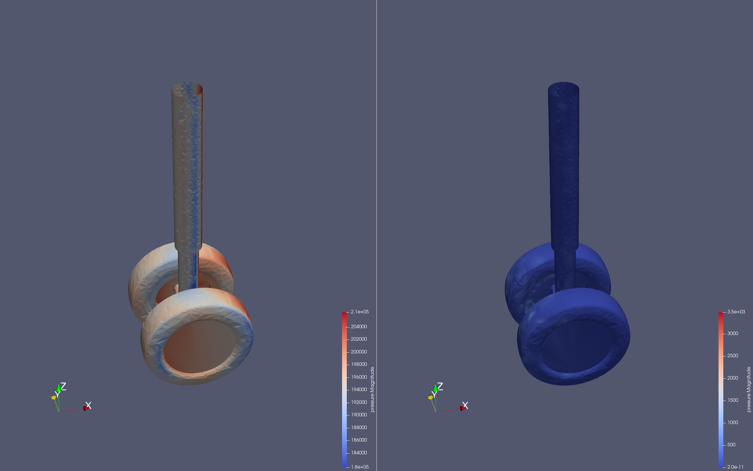
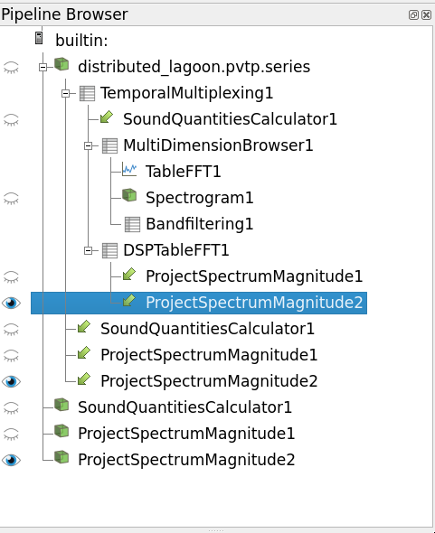
Visualization of low and high frequency spectrum magnitude projected unto the initial geometry

Finally, let’s compute the Mean Power Spectral Density

• Select the DSP Table FFT to make it active
• Add a Mean Power Spectral Density filter, Apply

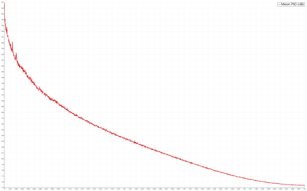
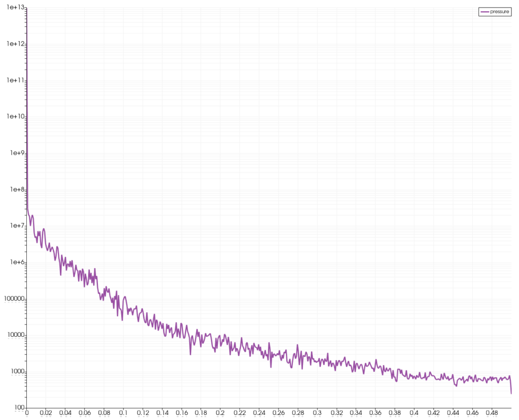
Visualization of the Mean Power Spectral Density

Please find a state file containing the results for these steps as well as a toy dataset compatible with it. Let us know if you would like to have access to the dataset used to generate the above screenshots.

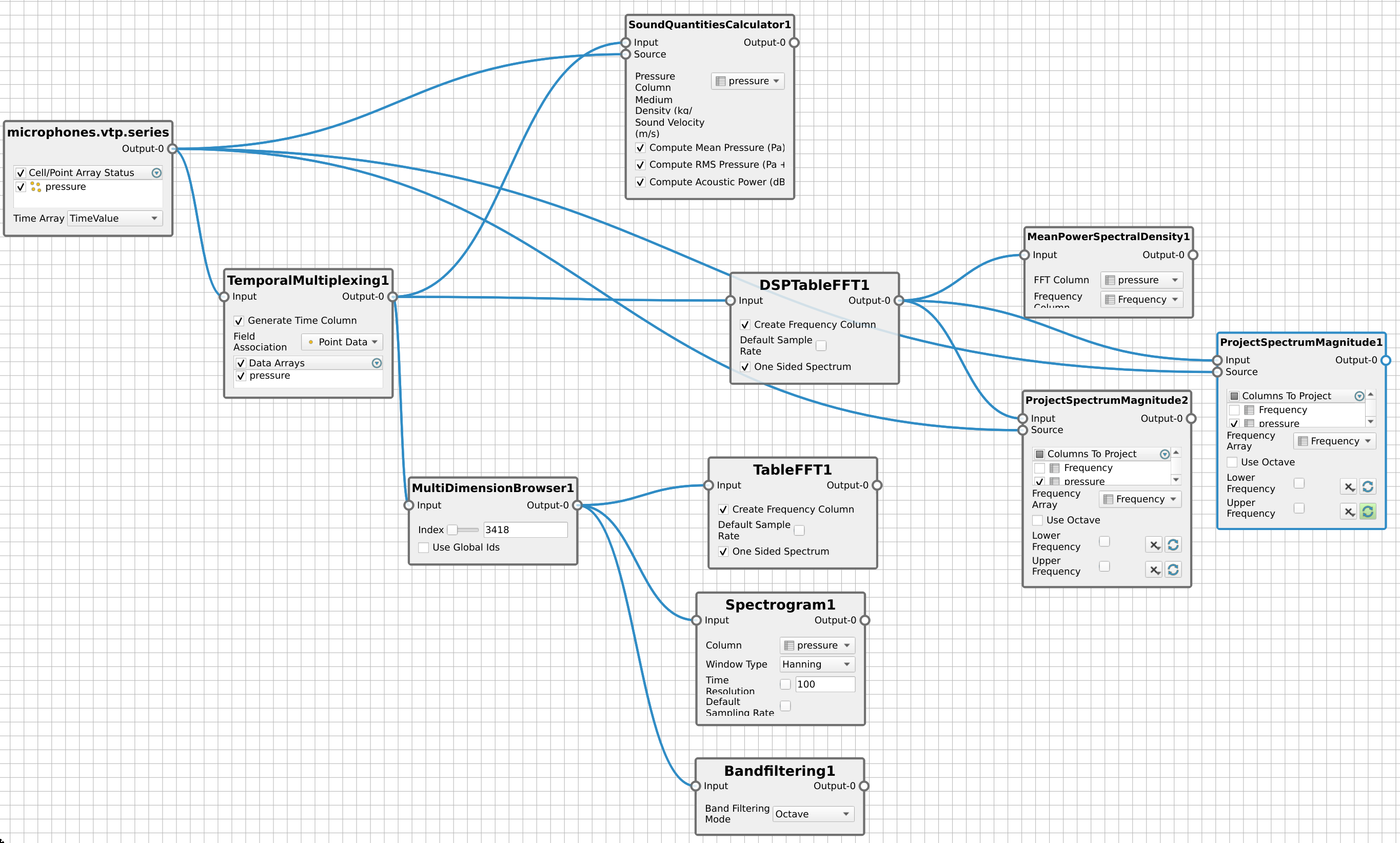
Illustration of a complete acoustic pipeline using the NodeEditor

Future improvements

This initial work on the DSP plugin has triggered a considerable amount of interest in the community and generated many avenues of prospective feature development and improvements.

Many acoustic processing algorithms could be added in order to provide with more tools for acoustic workflows, especially BeamForming.

Acknowledgement

This work was funded by the CALM-AA European project (co-funded by the European fund for regional development).

Datasets and help about implementation has been provided by MicroDB.

Help with reviews and datasets has been provided by KM Turbulenz Gmbh

Datasets provided by Airbus.