Exporting WRF model results in Structured Grid format (.vts) – A PARAVIEW direct import.

Kitware note: This is a guest blog from Marco Miani and Yiannis Proestos from The Cyprus Institute.
Glossary
WRF: Weather Research and Forecasting
.vts: VTK Structured data format
Introduction
In our previous post, we addressed how to import WRF-model data into the ParaView environment, to be easily and effectively visualised, which required some processing and data manipulation. Specifically, two crucial steps had to be followed:
- interpolate the model data (originally defined on a curvilinear gid) on a regular, rectangular grid, and generate a re-gridded netCDF file;
- (re-) assign the vertical coordinate by means of a programmable filter. By doing so, the proper vertical topology was restored.
This new approach, instead, skips these steps. The (x, y, z) triplets for volume variables are pre-processed in python, appended to the variable of interest (e.g., temperature, pressure, relative humidity, dust concentration) and directly exported as a .vts? format file.
Advantages
The advantage is that no programmable filter is needed when using ParaView. .vts files can be opened directly and their topology is consistent with the WRF model it is based on. Therefore, the process is “shape preserving” and provides something that is “plug and play”.
Under the hood
Original data is imported into python. The .vts file to be exported needs to have following dimensions, and in this specific order:
And must be bundled with its geographic coordinates (x, y, z):
Same applies for y and z. Their size and shape must be consistent.
Time is not explicitly included in this example and, in this post, this temporal dimension is treated as a simple filename matching a given pattern. For instance, the timestamp or its index, are appended to a series of .vts converted filenames. ParaView interprets that as a family of items belonging to the same event. Whilst the actual diagnostic variable has a 3-D structure, geographical coordinates do not. Therefore, they are stacked to make coordinates and variables consistent in size, vertical coordinate z (which happens to be space varying) is assigned at the same time.
To achieve this, the `evtk` python package (https://github.com/paulo-herrera/PyEVTK) is used. See below for a code snippet, illustrating how to achieve the processing.
Model topography
Amongst the numerous input files, the numerical model ingests land topography, to which meteorological variables must snap. This section presents and describes how structured data inherit the native model topology to allow and ensure that match.
All variables “start on top” of model-ingested, native land topography. For instance, the baseline of the data-volume representing air temperature, follows the terrain. The following figure shows how the bottom of the data-volume is partly “empty”, pre-allocating the space for the topography to compenetrate the data, by matching their spatial distribution.
A classic topological grid
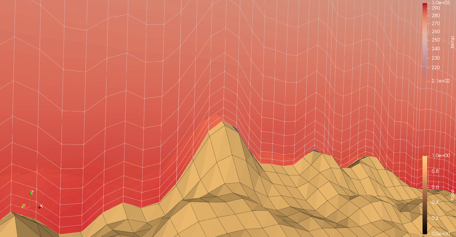
Variables gridlines (topography and air temperature) that contiguously match
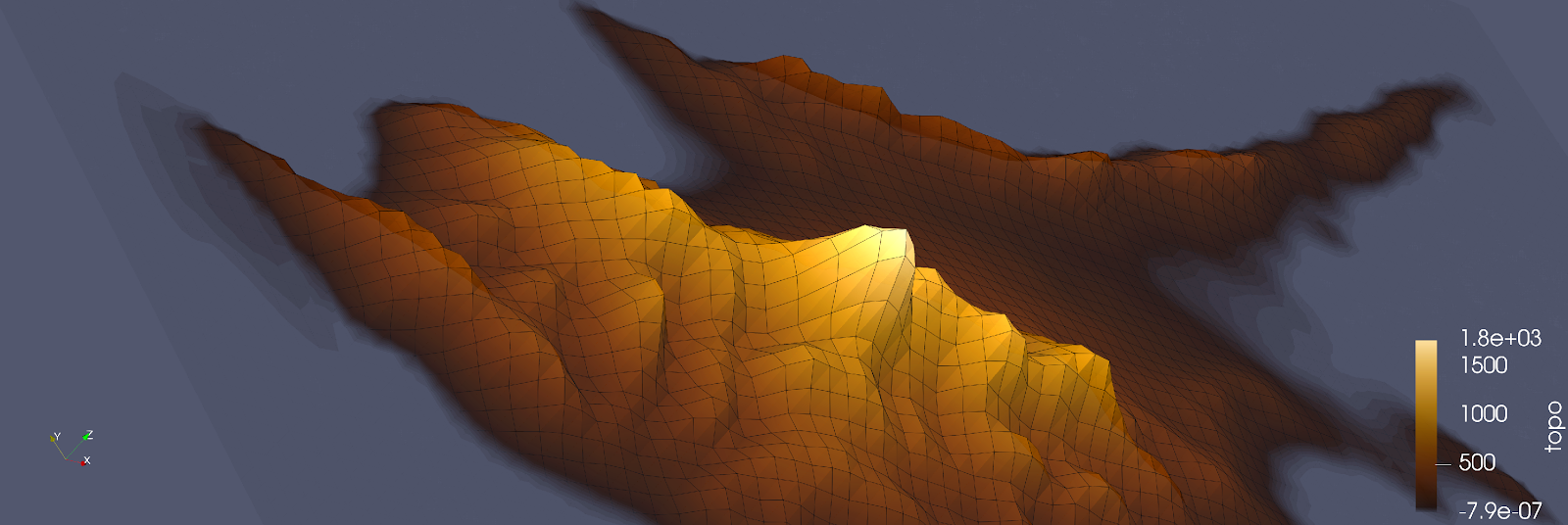
A detail of a model topography
Curvilinear grids
Curvilinear grids are herewith easily visualizable. The model consists of a recursively nested model domain. The smallest domain, due to its size, presents a small deformation. However, when plotting larger mother domains, the grid deformation is indeed visible.
This following image shows how the smallest domain is nested into the bigger mother domain. The numerical grid of former and latter domains, shown here as bounding boxes, presents different degrees of spatial deformation. This demonstrates how curvilinear grids can indeed be represented with exported .vts files.
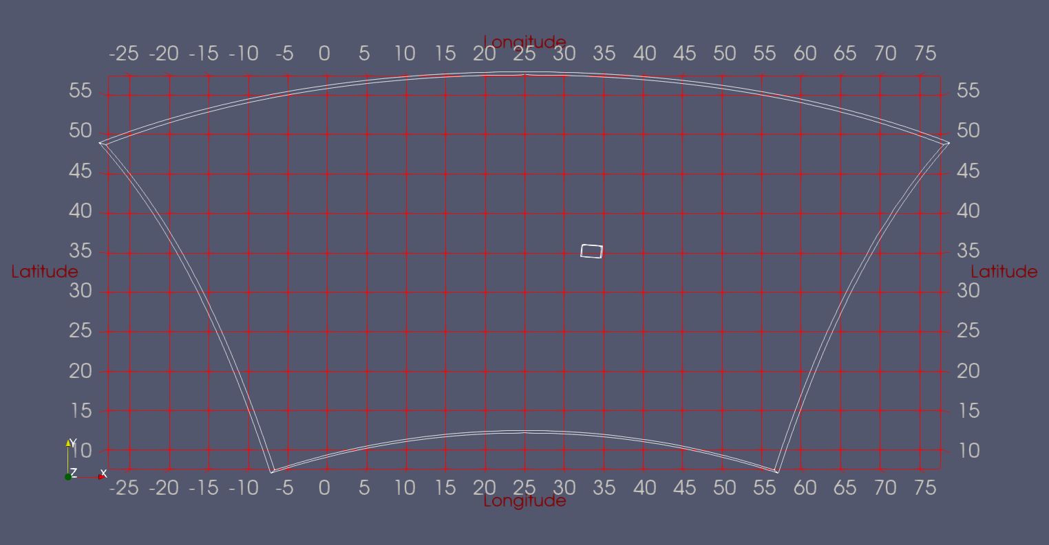
Small domain inside a bigger domain

The model setup, in particular the so-called telescopic nesting of the 3 model domains. The bigger, outermost domain, provides the nested ones with boundary conditions.
Results
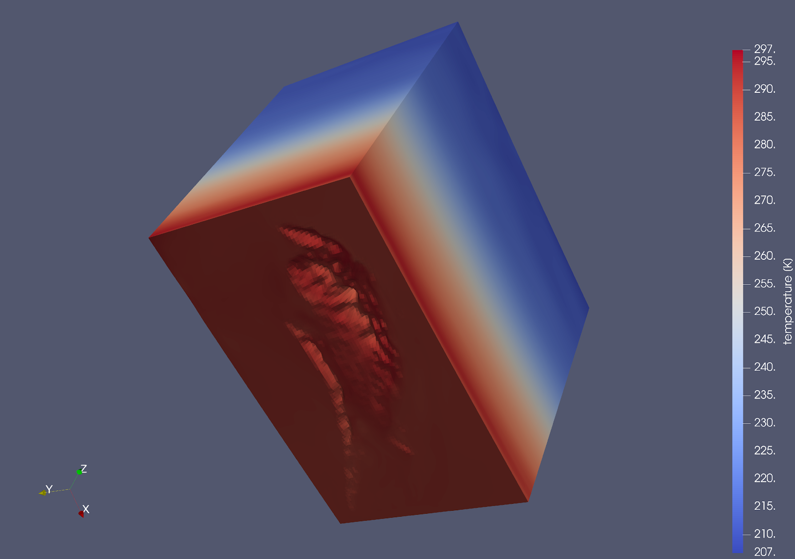
In light of all the aspects described above, the final result is a structured grid with associated scalar data, to which all the most common PV filters (e.g., slicing, threshold, subset, contour) can be applied. A complex data structure (WRF-generated) can now be visualised and crucial information contained in it can be easily extracted and inspected.
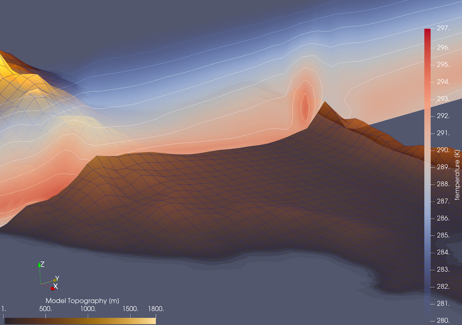
An image to show how the model is capable of capturing the formation of a warm air pocket on the leeward side of Pentadaktylos mountain ridge, a long, narrow mountain range that runs for approximately 160 km along the northern coast of Cyprus.
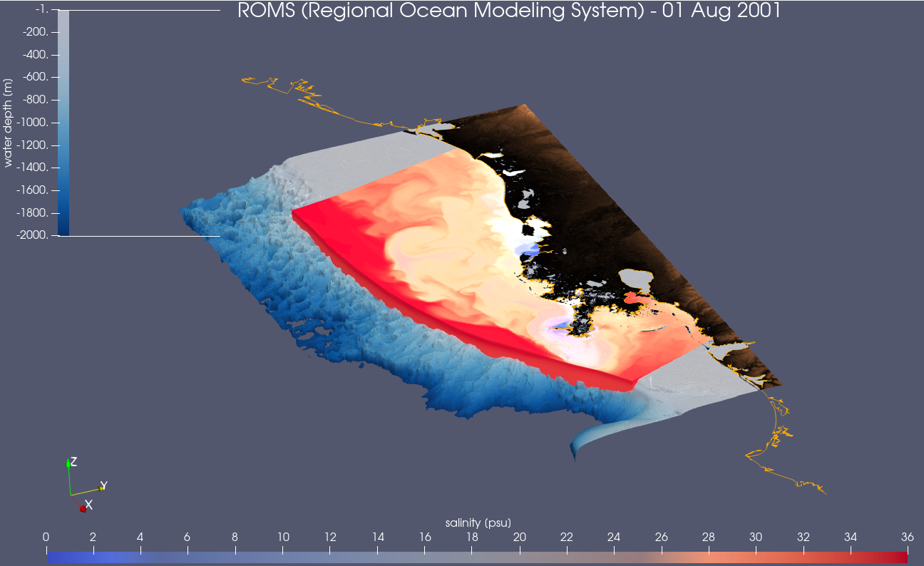
A practical Application: The Regional Ocean Modeling System
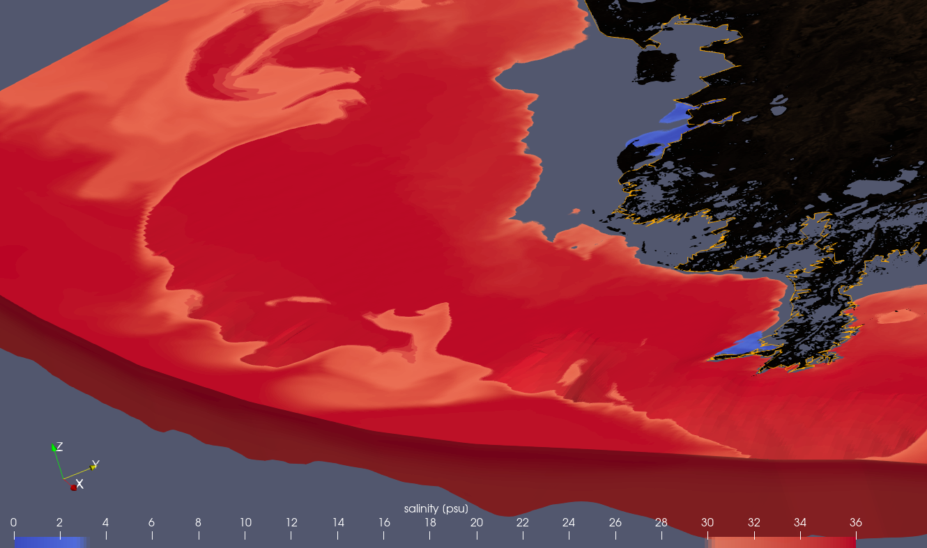
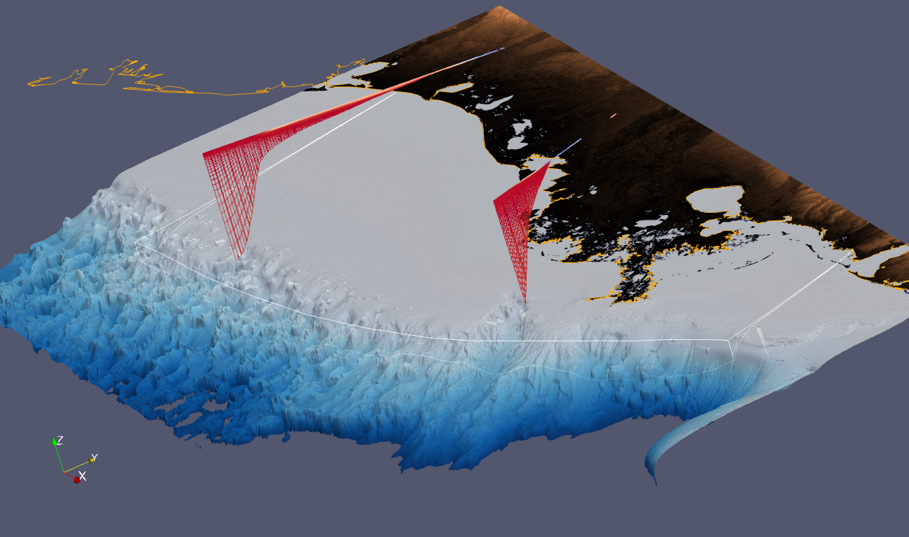
A demonstrative oceanographic data-set is available at https://docs.xarray.dev/en/stable/examples/ROMS_ocean_model.html. This data was pre-processed (computing and appending metric vertical coordinate, instead of sigma, terrain following coordinate; the method is described in the link above) and converted to .vts format. They show 3D salinity fields for the surrounding area of the Mississippi Delta, in the southern United States. A clear contract between fresh/salty water is visible, as well as the surface large eddies.
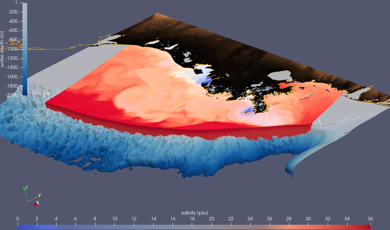
By extracting vertical slices of the dataset, it can be seen how the freshwater, less dense, ends up floating on the larger, saltier, denser water mass contained in the basin.

Code snippet
As an example, the python code used to manipulate ROMS model data is added to showcase the procedure:
'''
Author:
  Marco Miani
  Computational Support Specialist
  Climate and Atmosphere Research Center (CARE-C)
  The Cyprus Institute
  20 Konstantinou Kavafi Street, 2121, Nicosia, Cyprus
  Tel: +357 22 397 561 | Email: m.miani@cyi.ac.cy
  Web: cyi.ac.cy | emme-care.cyi.ac.cy

Version:
  11 Jan 2023

Content:
  Convert ROMS oceanographic data, namely salinity s(x,y,z), to vtk file
  Input ROMS data belong to in-built XARRAY tutorial dataset.

'''

import evtk as ev
import xarray as xr
import numpy as np

#=========================================================================
# Local parameters and their definition:
#========================================================================

#scale factor
z_factor = 0.001

#Where to save my data, on local machine
saveFolder = '/home/..somewhere.../ROMS/salinity'

#=========================================================================
# from https://docs.xarray.dev/en/stable/examples/ROMS_ocean_model.html
# Import ROMS data, as a test case example (and extract first timestep)
#=========================================================================
ds = xr.tutorial.open_dataset("ROMS_example.nc").isel(ocean_time=0)

#========================================================================
# Manipulate vertical sigma coordinates, as described in:
# https://www.myroms.org/wiki/Vertical_S-coordinate
#========================================================================
if ds.Vtransform == 1:
  Zo_rho = ds.hc * (ds.s_rho - ds.Cs_r) + ds.Cs_r * ds.h
  z_rho = Zo_rho + ds.zeta * (1 + Zo_rho / ds.h)
elif ds.Vtransform == 2:
  Zo_rho = (ds.hc * ds.s_rho + ds.Cs_r * ds.h) / (ds.hc + ds.h)
  z_rho = ds.zeta + (ds.zeta + ds.h) * Zo_rho

#Append coordinates to original dataset:
ds.coords["z_rho"] = z_rho.transpose()  #transpose seems to be xarray bug
#=========================================================================
#Pre-allocate, for variable "salt":
#=========================================================================
#Space coordin.:
x = np.ones(ds.salt.shape)
y = np.ones(ds.salt.shape)
z = np.ones(ds.salt.shape)

#Assign actual values for: x, y, z
for k in range(0, len(ds.s_rho)):
    x[k,:,:] = ds.lon_rho.values.T
    y[k,:,:] = ds.lat_rho.values.T
    z[k,:,:] = ds.z_rho.isel(s_rho=k).values.T
    print("Processing level {:2d} of {:d}".format(k+1, len(ds.s_rho)))

#========================================================================
# Actual salinity values:
#========================================================================
s = ds.salt.values #consistent in shape

#========================================================================
# Save to vtk, as gridded data (not point cloud!):
#========================================================================
ev.hl.gridToVTK(
      saveFolder, #where to save
      x,        #longitude
      y,        #latitude
      z_factor*z, #depth
      pointData = {'salt' : s}
)

print()
print(50*"=")
print("File saved:\n"+saveFolder)
print("(Vertical scale factor, set to {:1.2e})".format(z_factor))