Scientific visualization of Weather Research and Forecasting model output in Paraview
implementation of a tailored filter to restore the terrain following topology of native dataset.
Kitware note: This is a guest blog from Marco Miani and Yiannis Proestos from The Cyprus Institute.
Glossary
WRF: Weather Research and Forecasting
CF: Climate and Forecast
VAPOR: Visualization and Analysis Platform for Ocean, Atmosphere, and Solar Researchers
NCAR: National Center for Atmospheric Research
GEBCO: General Bathymetric Chart of the Oceans
PBL: Planet Boundary Layer
What is the motivation?
Weather Research and Forecasting (WRF) model generated climate data are enormous in size and complex in topological structure, which reflects the intrinsic properties of the physical process they intend to represent. Effectively visualizing its content i.e., unfolding the large amount of information contained in them and conveying the message in an understandable way, especially to the general audience, is crucial in scientific dissemination. In that spirit, this first post presents the implementation of a so-called Programmable Filter, within the ParaView environment. A second post present another, more generic approach. The aim of such filter is to reconstruct/restore the geometrical topology, also known as “terrain-following vertical levels”, allowing the visualization of scientific data with ParaView, and making use of the arsenal available within that environment to achieve the highest possible quality in visualization.
What do we have so far to visualize and inspect WRF climate data?
There exist a plethora of tools and software to visualize this specific type of data, intended for creating both static images ([1],[4]) or animating ([2]) the results, so to display the time-varying nature and capturing the temporal evolution of any given relevant physical process (e.g., cloud formation, wind intensification, effect of solar irradiance, accumulation of tracers, etc.). WRF model data are not CF-compliant (see [5] for more detail), and a dedicated (open-source) scientific visualization facility, called VAPOR, capable of ingesting these data effortlessly and without requiring the user to do any pre-processing, has been developed at NCAR ([2]). However, when compared to ParaView some features are still missing, the software is not (yet) as flexible and lacks features and flexibility to achieve that high-quality in bringing out detailed visual information. A dedicated Python package ([7]), very powerful and flexible, was developed too.
What is really happening under the hood?
If imported unprocessed, WRF model data are not displayed correctly as ParaView is not able to link WRF computed variables to the complex space-varying structure (elevation/altitude) of the vertical coordinate: eta levels. In atmospheric science, it is very common to have the data defined over p coordinate: this means that the vertical coordinate is pressure (typically log-distributed, and with units in Pa), instead of geometric height (above sea or ground level, with units in meters). The information describing the vertical coordinate (geometric height) is extracted and appended when pre-processing model results, re-gridded, passed along to ParaView, and thereafter extracted by the Programmable Filter. Thus, armed with this information, the filter programmatically retrieves that information, reassigns the “correct” vertical coordinate information (retrieving it from the ancillary variable) and, by doing so, restores the “correct” vertical topology (geometric, in meters above a given reference). This returns a global picture that is more understandable and, more importantly, directly comparable/stackable with surrounding terrain. This last aspect, greatly facilitates the comprehension and interpretation of climate model data. See below for a breakdown of the code of the programmable filter.
Preparing and preprocessing the data in a way that ParaView likes.
In addition to the step mentioned above, another step needs to be taken care of before importing the data within ParaView environment and actually applying the filter: original data need to be re-gridded, through interpolation, on a regular (rectilinear/latlon) geographic grid. The (horizontal) computational grid over which WRF crunches numbers and carries out its magic computations is (usually) a projected curvilinear one. This means that grid-lines are not straight lines or, in other words, latitude and longitude are not linearly independent. Again, in other words, longitude ends up being a function of latitude, and vice versa.
The conversion process between these two topologies is called interpolation. For the time being, it is achieved outside the ParaView environment.
In this intermediate step, data are transformed on a new regular geographic grid, the total number of re-gridded variables to be included is reduced (a selection of the available 396 variables, contained in the original data-set) and a time-marching loop interpolates and appends the user defined information, at each time-step. The result of all this is a netCDF file that is ready to be ingested into ParaView.
And what about the results? What do they look like? How are they different?
As mentioned above, if imported unprocessed, model data present unphysical intersections with local terrain (e.g., “data through mountains”). This is not realistic as the model uses a “terrain-following” configuration. The original vertical dimension of the (already pre-processed/re-gridded) model data is lev (or bottom_top, in native WRF coordinate system). This sequential index is mistakenly considered by ParaView as geometric elevation. Omitting for an instant that the unit of measure of the index (meters? kilometers?) would not make the slightest sense, the real problem behind this assumption is that the spatial distribution of height iso-surfaces (z), is not constant over space. In other words, that means level-heights are not flat laminae. Instead, they adhere to underlying topography and (the amplitude of) their deformation decreases with geometric height (almost flat at the top, and deformed at ground level).
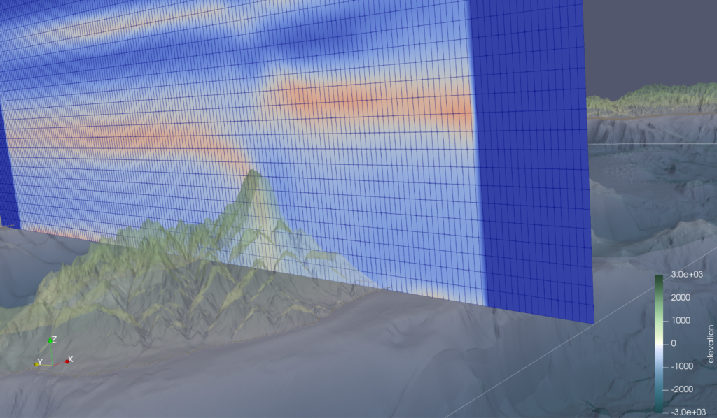
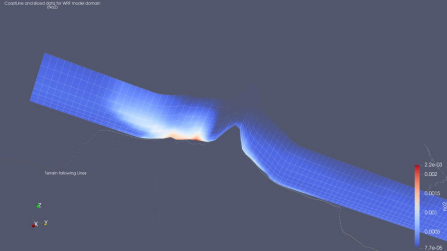
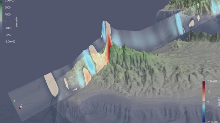
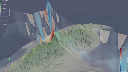
After applying the filter, data is actually “following” the terrain and the problem of data compenetrating the terrain is solved. Now, the data are actually mapped where they are supposed to be. Figure 1 shows the result of applying the Programmable Filter. The slice ‘following along’ the terrain cross section can be seen, across and above Mount Troodos, in Cyprus.
A slight mismatch between (sliced) data and topography can still be seen. This is because we decided to use high-resolution topographic data, sourcing it from GEBCO. Our WRF model runs on a computational grid, where we have chosen a horizontal grid spacing of approximately 2km. The topography is gridded at 250 meters. We could have easily used the topography file contained in the model results (deriving, in turn, from model output) but for the sake of appearance, we decided to overlap our data to an alternative (open-source) topographical dataset.
Why would you study the lowest layer of the Atmosphere? Nobody interested in high-altitude meteorology would ever care about some slight mismatch at ground level? So, why bother?
First off, for consistency reasons: right is right. Furthermore, for this specific case, WRF model runs on our HPC on a daily basis, specifically for Cyprus, and high-resolution output is constantly generated (on average, we generate 10 GB of data each day). The Environmental Predictions Department of the Cyprus Institute, along with the Cyprus Dept. of Meteorology, use this valuable information to conduct their research which includes (but is not limited to) low altitude and within the PBL, in-situ measurements, using tailored sensors mounted on our fleet of UAV and sondes.
Commented code of the programmable filter
# Recover the inputs
input     = self.GetInputDataObject(0, 0)
output  = self.GetOutputDataObject(0)

# Copy the input into the output
output.ShallowCopy(input)

# Create a new set of points
newPoints   = vtk.vtkPoints()
numPoints   = input.GetNumberOfPoints()

# Print the current time step, for display only
t = self.GetInputDataObject(0,0).GetInformation().Get(vtk.vtkDataObject.DATA_TIME_STEP())
print("time: ",t)

# Recover the elevation data
q     = "zk"    # or "zLev" or "z", depending on the name used to store the variable containing vertical topology
input0  = inputs[0]
zlev    = input0.PointData[q]
print(zlev) #comment or uncomment to print out elevation on terminal


# Foreach gridpoint in my domain:
for i in range(0, numPoints):
    # Extract coordinates
    coord   = input.GetPoint(i)
    x, y, z   = coord[:3]

    # Replace the z coordinate by the elevation data
    z     = zlev[i]

    # Insert new points with terrain following
    newPoints.InsertPoint(i, x, y, z)

# Set the points on the output
output.SetPoints(newPoints)
Find the original code here: https://drive.google.com/file/d/1COGonQ5C9hOe7zP13rwRn3LIFKsPSP0B/view?usp=sharing
Please note the current code could be simplified into a calculator filter with the following expression and “Result Coordinates turned on: `coordsX*iHat+coordsY*jHat+zk*kHat`. However, with real data, one may have to switch arrays or do more complex computations in order to recover the actual elevation data, hence using a programmable filter to make it more practical.
About the authors and The Cyprus Institute:
Marco Miani
https://www.cyi.ac.cy/index.php/care-c/about-the-center/care-c-our-people/author/1084-marco miani.html
Yiannis Proestos
https://www.cyi.ac.cy/index.php/care-c/about-the-center/care-c-our-people/author/115-yiannis proestos.html
Climate and Atmosphere Research Center – CARE-C, The Cyprus Institute
Unmanned System Research Lab:
References and Links:
(1) NCL – Interpreted language developed specifically for scientific data analysis and visualization, last accessed on July 4th, 2022 https://www.ncl.ucar.edu/index.shtml (2) NCAR- VAPOR official webpage, last accessed on Jul, 4th, 2022 https://www.vapor.ucar.edu/ (3) CF (Climate/Forecast) convention: vertical coordinate. https://cfconventions.org/cf conventions/cf-conventions.html#vertical-coordinate, last accessed on July 4th, 2022. (4) Xarray, a python-based package for multidimensional data
https://docs.xarray.dev/en/stable/, last accessed on July, 4th, 2022.
(5) CF conventions https://www.earthdata.nasa.gov/esdis/esco/standards-and references/climate-and-forecast-cf-metadata-conventions , last accessed on July 4th, 2022. (6) The General Bathymetric Chart of the Oceans (GEBCO) – publicly available bathymetry data sets. https://www.gebco.net/ Last accessed on July, 4th, 2022.
(7) A collection of diagnostic and interpolation routines for use with output from the Weather Research and Forecasting (WRF-ARW) Model, https://wrf-python.readthedocs.io/en/latest/ , Last accessed 5th July, 2022