Recent improvements in Georeferenced SLAM in LidarView

This blog covers the main improvements added to LidarView and the SLAM library to help with building georeferenced maps and shows the new possibilities offered. 

We will first cover the basic concepts involved regarding SLAM and the used external sensors, then go through the various updates that help users build such maps.

Primer on SLAM and georeferencing

SLAM basics

In a nutshell, the SLAM algorithm iteratively estimates relative poses and maps of its surroundings as the sensor moves in its environment by registering new frames on the dynamically built map. 

It is wrapped in LidarView through a filter that takes as input the LiDAR frames and outputs keypoint maps and estimated trajectories.

It can also optionally ingest extra information from external sources to make it more robust and accurate.  

More details about the SLAM library itself can be found in our previous blog post: https://www.kitware.com/lidar-slam-spotlight-on-kitwares-open-source-library/

External sensors used in SLAM

As stated previously, adding information from external sensors can improve the results of the SLAM significantly depending on the scenario and the desired output. The main external sensors used in the SLAM are the following:

• Wheel odometry: usually based on wheel tick counts, this provides an extra constraint in the movement direction and is particularly useful in cases with an uncertainty in that direction, such as a corridor / tunnel or a highway. 
• IMU (Inertial Measurement Unit): provides longitudinal acceleration and rotational velocity, usually at a high frequency. It is particularly useful to compensate for intra-frame fast motion, such as when the sensor is handheld.
• GNSS (Global Navigation Satellite System): provides georeferenced positions with various degrees of accuracy, in particular depending on whether it is relying on RTK and / or has been post processed (PPK).
• INS (Inertial Navigation System): provides full 6DoF georeferenced poses using motion sensors combined with GNSS receivers. 

Georeferenced positions need to be projected to local cartesian coordinates, see the PROJ project regarding this topic.

More details on the expected data are available in the SLAM documentation’s dedicated section.

They can be used at various stages of the SLAM process:  

• Ego-Motion prediction
• A weighted constraint for local SLAM optimization
• Point Cloud undistortion
• Pose Graph for post processing using all constraints

In the pose graph, links represent constraints derived from iterative registrations and external sensor measurements, together with their associated uncertainties.

Additional constraints may also be introduced, such as loop closure constraints or known passage points.

Integration of external maps in ParaView / LidarView

ParaView’s GeographicalMapFetcher source (from GeographicalMap plugin) allows users to download background maps from different providers and load them in the ParaView environment.

The implemented providers are:

• Google Maps (requires an API key)
• MapQuest (requires an API key) 
• OpenStreetmap (recently added, does not require an API key, but does not contain aerial imagery)

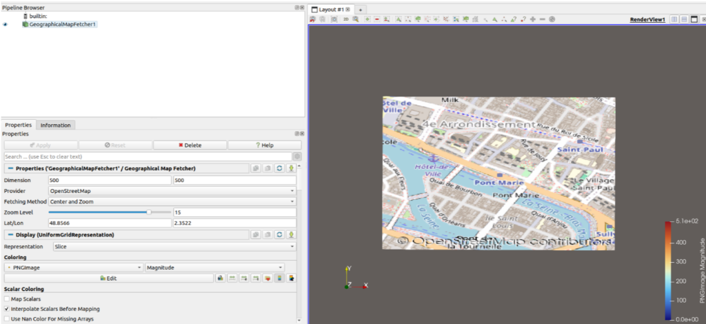
Map fetched from OpenStreetMap (Paris’ Presqu’Ile) 

How to integrate external sensors

Previously, external sensor data handling in the SLAM was done only internally and csv files with expected formatting had to be created in order to feed it to the algorithm. See this guide for more details on expected inputs. 

This is still functional, but we have also added a more “LidarView-style way” of doing this by adding a reader for external sensors, to be connected to the SLAM filter as a secondary input.

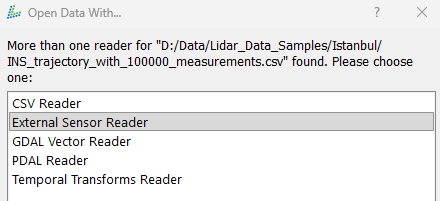
When opening a CSV file in LidarView, you now have the option to choose the External sensor reader that will output data i the format it is expected by the SLAM depending on the type of sensor you are using. This reader also allows users to define the rigid transformation between the LiDAR or base frame and the external sensor. Additionally, you can select a unit, which will be automatically converted to the one required by the SLAM algorithm. 

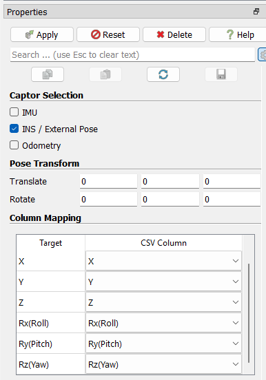
Interface of the custom external sensor reader

The importance of calibration and how to refine it

In order to use the measurements from an external sensor efficiently, the extrinsic calibration (e.g. relative pose to LiDAR sensor) must be known. An inaccuracy on it would lead to biases in the measurement integration.  

We have therefore developed a filter to help estimate the calibration between full 6DoF poses (such as ones extracted from an INS sensor) and a LiDAR sensor. 

The approach is based on a point cloud aggregation filter that uses the external pose transformed into the LiDAR coordinate system. The accuracy of the calibration directly impacts the results: the more precise the calibration (minimizing pose errors), the thinner and more accurate the reconstructed surfaces of the environment will be.

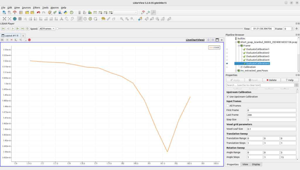
To quantify this, the filter will perform an aggregation of the LiDAR frames (with configurable parameters for steps and voxel size). For each aggregation set of calibration parameters, it counts the number of filled voxels.The assumption is that the more accurate the calibration is, the smaller number of voxels shall be filled with that method (this is especially true for rotational parameters that impact the point positioning the most).

The figure below presents an evaluation of the yaw component of the calibration between the LiDAR and the INS using the Istanbul Open Dataset. What can be seen is that modifying that value away from its real value increases the amount of voxels filled by the aggregation.

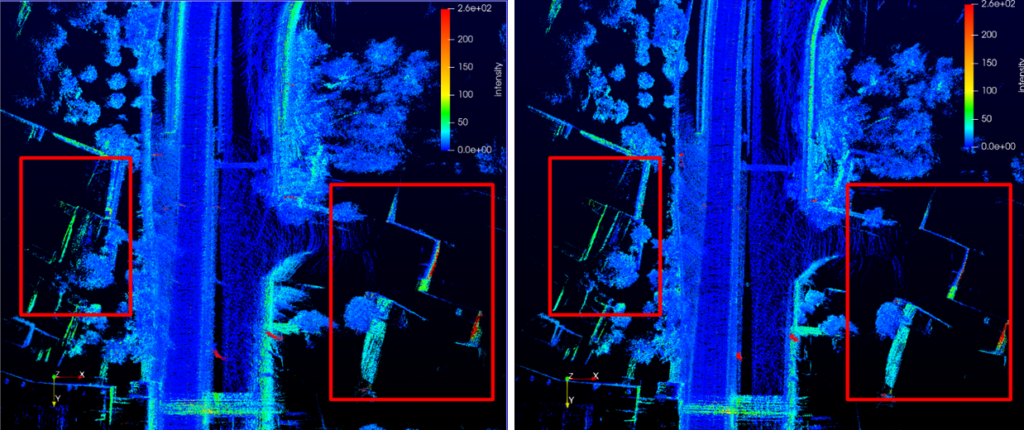
To illustrate the impact of the calibration, we aggregated the LiDAR frames along the trajectory measured by the INS. The left image below shows the resulting map using the original calibration (LiDAR-to-INS transformation), while the right image shows the map with an improved calibration. We highlight some areas where we can clearly observe an improvement on the map such as wall thickness reduction or misalignment correction.

Note that this is preliminary work and should not yet be considered to be an automatic reliable procedure. It also requires a decent initial estimate for the calibration. Main improvements needed to reach that point are:  

• Application of this method across various motions (both in terms of rotation and translation ) and various environment structure
• Automatic minimization procedure of the parameters (current implementation is a simple brute force search in the parameter space)

Added support for multiple sensors

We recently added the support of multiple LiDAR sensors in our SLAM library, enabling the possibility for a broader field of view. 

Support for multiple LiDAR inputs was previously already available in our ROS wrapper. This capability has now been integrated directly into the SLAM filter in LidarView.

The principle is to extract keypoint features independently from each LiDAR frame and transform them into a common reference frame (base frame). This allows SLAM to treat observations from different sensors as a unified representation of the environment.

To use this feature, users can follow these steps:

• First, apply a transform to each LiDAR so that its point cloud is expressed in the base frame.
• Second, select all frames and apply the Group Datasets filter to combine them into a multiblock dataset in LidarView
• Third, apply the SLAM filter to the grouped dataset.

At each timestep in the LidarView pipeline, the system checks whether a new frame has been received from each sensor and whether its timestamp has been updated since the last processed frame. The frames are then passed to the SLAM module only when all expected inputs are available and updated, or when a timeout is reached.

Map guided trajectory correction 

Once the trajectory is displayed in a geographic context, small offsets become easy to spot near clear landmarks (intersections, tunnels, road edges). 

To correct them without restarting, the SLAM plugin now supports manual trajectory anchors!

These steps let you quickly apply a manual correction in LidarView:

• Enable the Pose Graph option in the SLAM plugin and choose to “Use manual position constraint”
• Pick a trajectory pose you want to adjust.
• Using an interactive handle, you can easily set a target position in the geographic frame
• Click Append to Table to add the anchor (add a couple more if you want the correction to be better constrained).
• If you want to avoid the whole trajectory “sliding” globally, enable a fixed pose anchor as a stable reference.
• Finally, just click Optimize Graph to run the global optimization and update the trajectory.

With the map as a reference and these manual anchors, your trajectory can be brought back to where it should be in the real world.

The video below shows how we can adjust the SLAM trajectory based on an OpenStreetMap tile to make it fit to the road where the car was driving. The user inserts known passage points from the map overlay to add them as a constraint to the SLAM pose graph, then triggers the optimization.

A similar workflow can be used in cases with known passage points to ensure a coherent trajectory. For example if you have a robot in a warehouse that stops at known stations.

Use satellite data to colorize the point cloud

To go beyond displaying a basemap, LidarView now includes a new filter (ImageColorToPointCloud) to colorize point clouds using aerial imagery (or virtually any georeferenced image layer).

The filter takes two inputs:

• A map with RGB information in the form of a structured grid or image data 
• Georeferenced LiDAR point cloud 

It outputs a new point cloud where each point is assigned an RGB color sampled from the map at its corresponding geographic location.

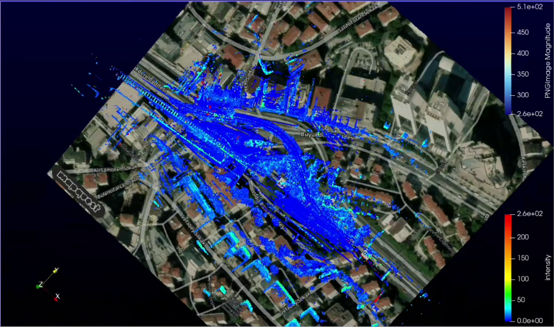
The video below shows how to use satellite data (from MapQuest) to color a georeferenced 3D map built with a LiDAR sensor, fused in the SLAM with an INS device.

What’s next? 

There are still multiple paths for improving these features to make georeferencing point clouds easier and more accessible. These include:  

• Automation of calibration determination and associated checks on datasets
• Automation of external map retrieval based on coordinates 
• Automatic detection of drift based on external maps 
• Add road and road surrounding information on the maps through:  pothole detection, curb localization, power line segmentation…
• …

Conclusion

We have shown in this blog post multiple tools to make georeferenced SLAM easier and more complete in the open source LidarView environment.  

Our goal is to enable these capabilities for relevant systems, making it adjustable to each user’s needs and allowing the addition of new functionalities in the open source ecosystem so that it can be used as a base for many applications using georeferenced 3D reconstruction, as well as adding intelligence on top of such data. 

If you are interested in developing such an application, please contact us to see how we can help you!