VTK as a Metrology Tool for 3D Reconstruction

In the 3D reconstruction domain, an important step is measuring the quality of generated models. Often, this step is done subjectively and can lead to poor estimates and regressions.

A better approach is to use metrology tools to compare reconstructions against a ground truth using objective metrics.. We present a pipeline leveraging VTK to perform this comparison between a 3D reconstruction from images and a high quality 3D model that will serve as the ground truth.

For the ground truth, there are typically two cases. Either you have a CAD model of your reference and want to measure the difference between the real data and that model, or you need to scan a reference piece with a high-accuracy setup (usually based on laser scanning). It is important that this setup has precision that is an order of magnitude higher.

3D Reconstruction Methods

In computer vision, there are currently two main methods for reconstructing objects in 3D from images without realtime constraints. The first method is called structure from motion (SfM), which finds similar patterns across different images of the same object using descriptors. Then, camera positions and/or intrinsics are estimated using the essential matrix that models each image pair. A typical approach for this is the 8 Points algorithm.

Running the SfM algorithm produces a sparse point cloud and camera positions/calibration for each image with associated patterns.

The second method is called Multi View Stereo (MVS), which uses pairs of images as independent stereo problems that are then combined into a single dense point cloud. To work correctly, this algorithm needs to know camera positions and intrinsic parameters, which are outputs of SFM.

Common Tools for Photogrammetry

COLMAP, an open source 3D reconstruction software, offers an easy way to run a two steps pipeline (combining SfM and MVS) to create a dense point cloud and is usually considered the most advanced tool for this task. There are many settings to constrain the reconstruction, but for a quick start, you can use the automatic reconstruction button and select the directory that contains all your images.

MVS is very computationally intensive and scales quickly with the number of images and their resolution. Depending on the output requirements, you can lower image resolution for faster results.

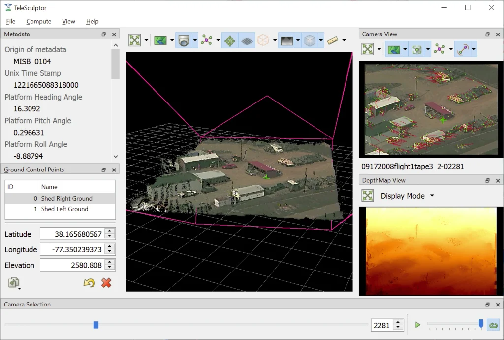
Kitware has developed Telesculptor, which performs SfM and MVS in a similar fashion, specifically tailored to turn aerial imagery into 3D geospatial models. It adds functionality specific to this use case, such as GNSS pose extraction from metadata, using ground control points.

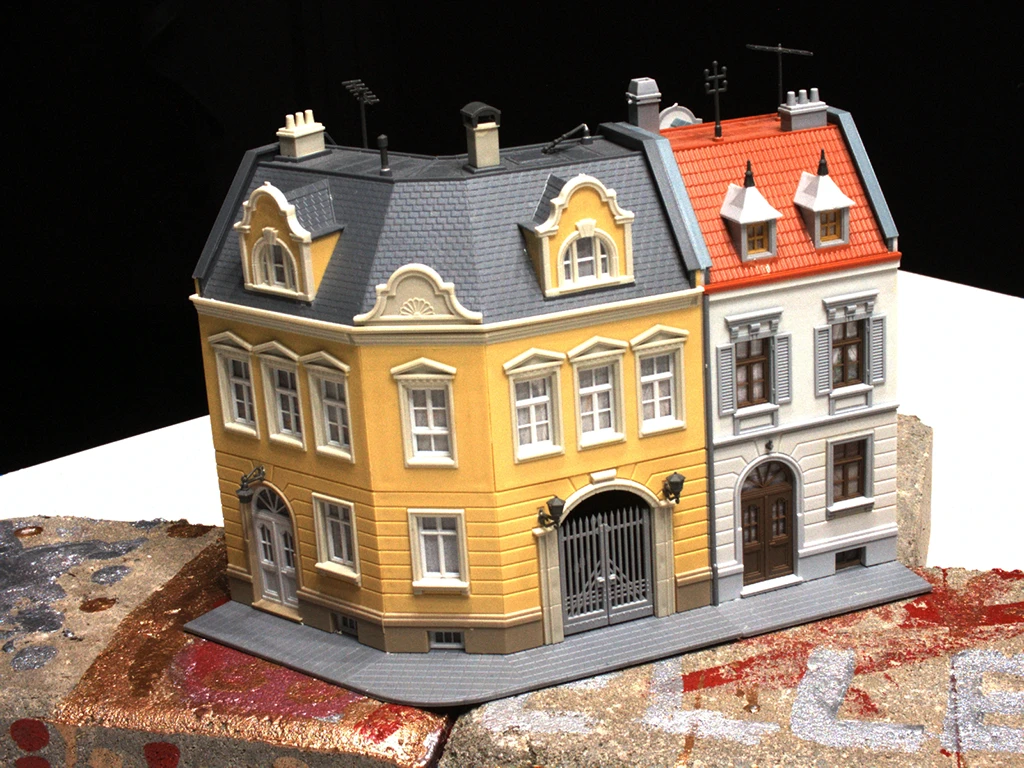
In this blog, the reconstructions as well as the ground truths are taken over from the DTU Robot Image MVS Data Set – 2014 dataset (we took “scan6” from the “SampleSet”).

Metrology Methodology

To compare generated reconstructions, we need meshes of our reconstructions and the groundtruth reference. We then need to align the models. Because they come from different sources, they are probably not captured with exactly the same position or rotation. A good way to do this is to use the Iterative Closest Point (ICP) algorithm.

Once perfectly aligned, we can compute the distances between the two surfaces at each point. Then, we can derive different metrics and visualizations of the errors for a better understanding.

VTK Implementation

VTK is the ideal tool to implement such a solution because of its filters and graphical capabilities.

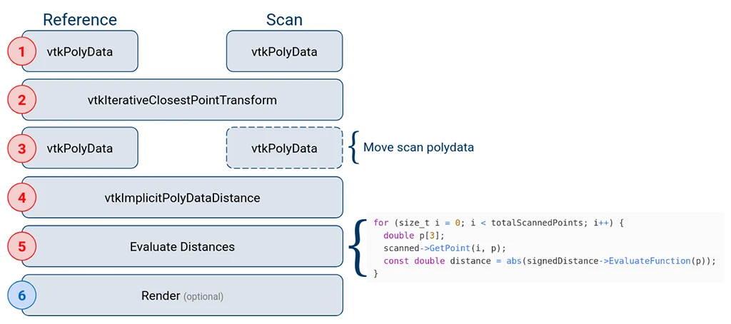
The metrology pipeline can look like this:

• Import models to compare and convert them to vtkPolyData
• Run the vtkIterativeClosestPointTransform filter
• Move the source object using the ICP results.
• Set reference polydata as input to vtkImplicitPolyDataDistance filter
• Call the EvaluateFunction(p) method for each point p.

The pipeline produces a signed distance, which you can square, take the absolute value of, or simply keep as-is to show distance direction.

Results can also be stored in a vtkDataArray and associated with scanned model point data for metric computation and visualization.

Results

We can compare two different MVS algorithms using this VTK pipeline.

The first reconstruction method implements [1] (Efficient large-scale multi-view stereo for ultra high-resolution image sets, E. Tola., et al). The second is based on [2] (Using multiple hypotheses to improve depth-maps for multi-view stereo, N. D. Campbell., et al).

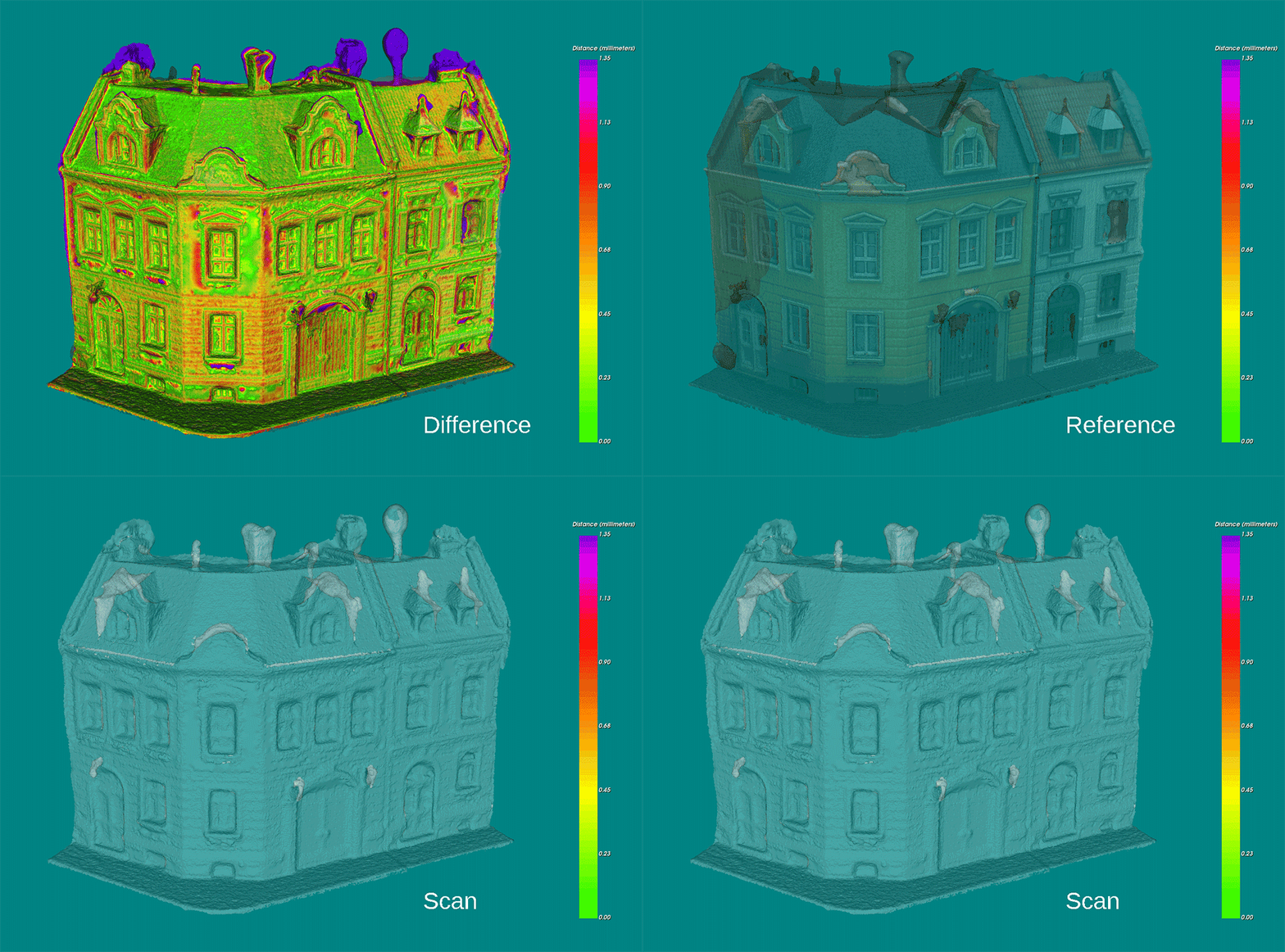
The first reconstruction (left) has a mean absolute error (on 85% of closest points) of 0.27mm, while the second (right) has 0.45mm of MAE. Raw number error measurements are useful as a simple comparison criterion, but they do not always tell the whole story.

Visualizing the distribution of the errors gives us a better understanding of where the algorithms fail and how they behave on the geometry.

In the example below, we can see that the most important errors in the second reconstruction are on the building edges and the slabs on the floor, where high spatial frequencies are found. The second reconstruction generates a geometry with an amplitude too large, whereas the first one smooths it out.

We can also see additional artifacts generated on the roof, particularly in areas with low contrast with the background.

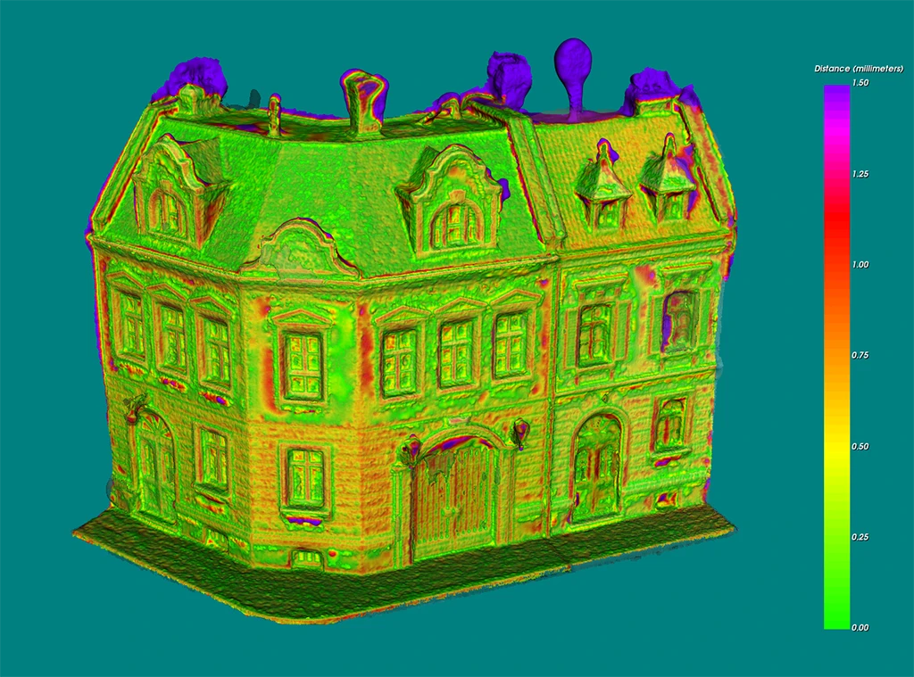
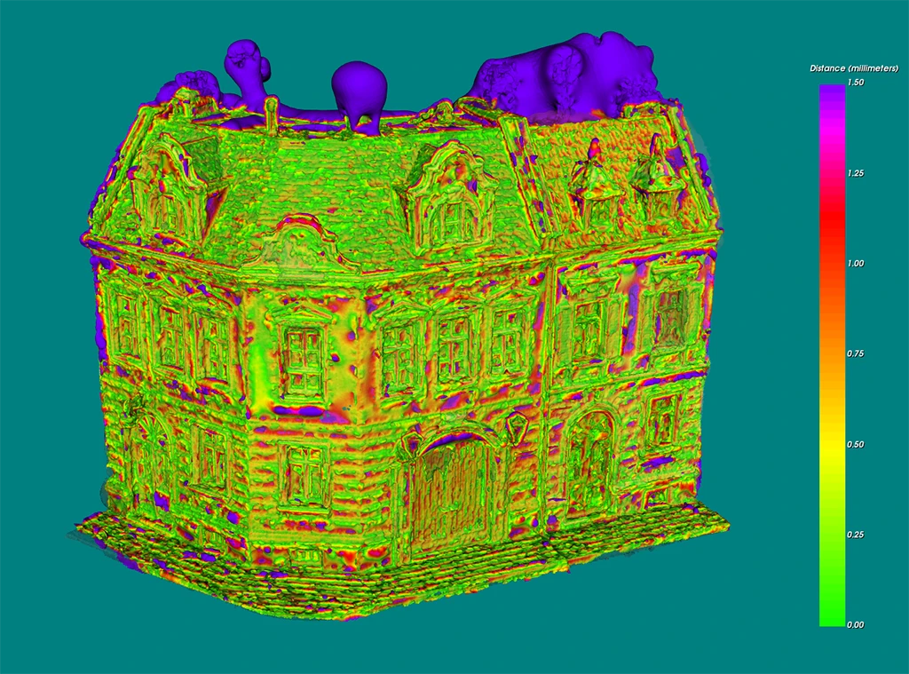
Left: Errors for 3D reconstruction with method [1], Right: Errors for 3D reconstruction with method [2], Bottom : example input image

This type of visualization can be extended to any 3D model that needs to be compared to a reference.

A possible application could be to perform a 3D scan of each piece coming off a production line, compare the 3D scan with a reference, and quickly visualize where the deviations are. This allows the operator (or a machine learning model) to judge the criticality of such deviations.

For instance, a deviation in the geometry of an electronic board may either mean that a weld is incomplete, or that a component has simply moved relative to the reference without functional impact.

This pipeline shows how we can combine expertise in Computer Vision and Scientific visualization to extract information from reconstructions of real world objects.

Do you see a use case where a similar approach could be applied?

Contact us to discuss how we can help you integrate this into your workflow.

References

Scans and reference meshes were produced using Screened Poisson Reconstruction on pointclouds from the DTU Robot Image MVS Data Set – 2014. The dataset is presented in this paper [5].

[1] Tola, Engin, Christoph Strecha, and Pascal Fua. “Efficient large-scale multi-view stereo for ultra high-resolution image sets.” Machine Vision and Applications 23.5 (2012): 903-920.

[2] Campbell, Neill DF, et al. “Using multiple hypotheses to improve depth-maps for multi-view stereo.” European conference on computer vision. Berlin, Heidelberg: Springer Berlin Heidelberg, 2008.

[3] Schönberger, Johannes L., et al. “Pixelwise view selection for unstructured multi-view stereo.” European conference on computer vision. Cham: Springer International Publishing, 2016.

[4] Kazhdan, Michael, and Hugues Hoppe. “Screened poisson surface reconstruction.” ACM Transactions on Graphics (ToG) 32.3 (2013): 1-13.

[5] Jensen, Rasmus, et al. “Large scale multi-view stereopsis evaluation.” Proceedings of the IEEE conference on computer vision and pattern recognition. 2014.