When True Negatives Go to Infinity: A Journey Through Metrics, Proofs, and AI

This blog post is a story that starts with a small observation about object detection. It ends with a formal Lean4 proof and a connection to ecology. Along the way, several people (and, more recently, LLMs) helped me contextualize and improve my observations.

For readers who want a refresher before the story gets going: this post relies on the ideas of true positives, false positives, false negatives, true negatives, precision, recall, the Matthews correlation coefficient, and the Fowlkes-Mallows index, all of which are defined in the glossary at the end.

At a high level, this story spans several years. In 2019, I noticed that as true negatives go to infinity, the Matthews correlation coefficient approaches the geometric mean of precision and recall, also known as the Fowlkes-Mallows index. In 2022, I wrote up a proof. In 2025, I formalized it in Lean4. And in 2026, I found earlier work showing that the same relationship had already been observed under different terminology. While the result isn’t novel, the connection, framing, and formalization are. This is the story behind the paper: “The MCC approaches the geometric mean of precision and recall as true negatives approach infinity.”

Scoring Object Detection

Back in 2019, I was thinking a lot about how to compute evaluation scores for object detection algorithms. Everyone seemed to have their own way of doing it, and the existing standardization was weak. I wanted to take a stab at improving the tooling landscape around the problem, which meant I needed to deepen my understanding.

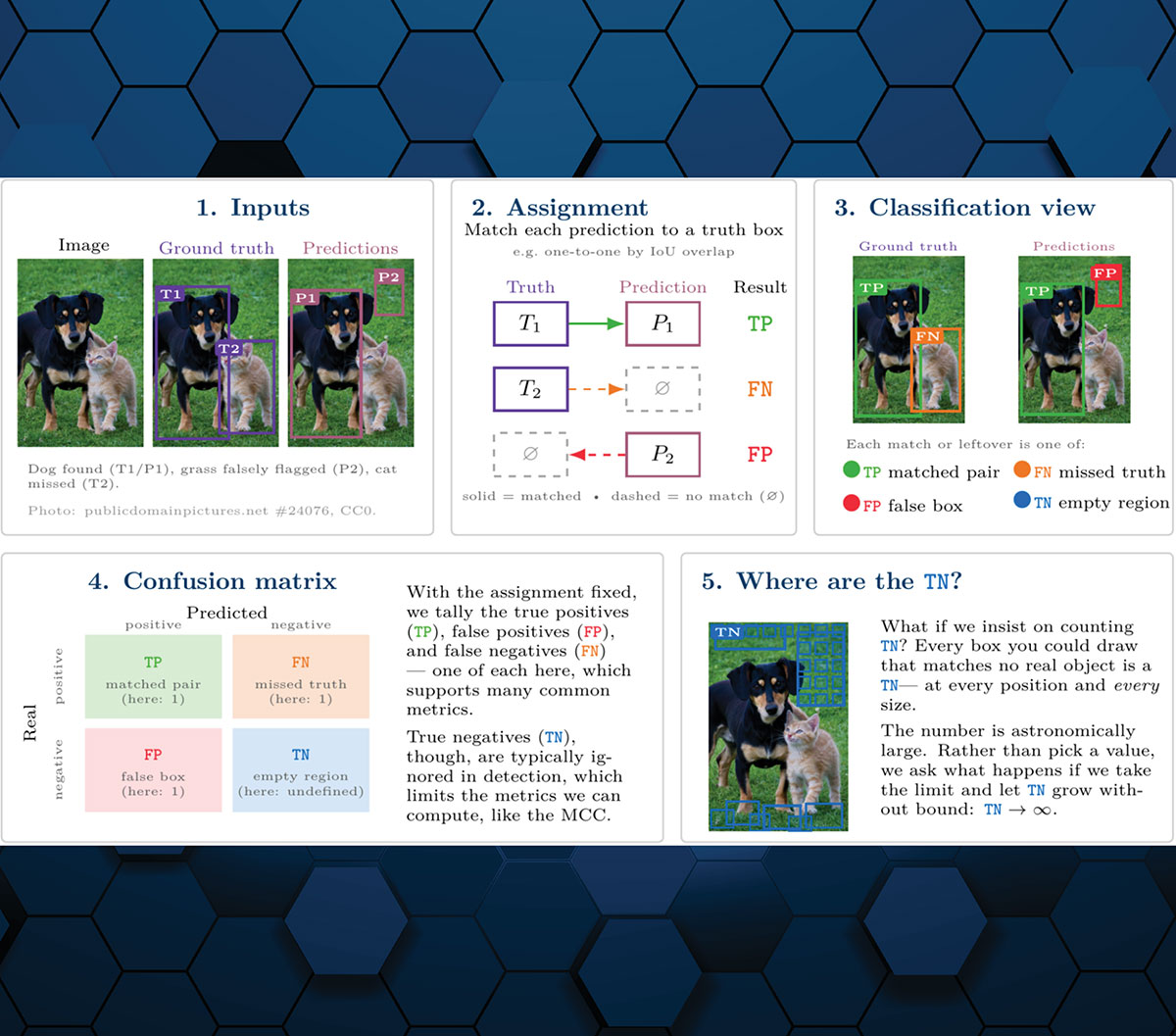
The concept that made the problem click for me was realizing that detection scoring can be decomposed into two simpler components. First, an assignment algorithm matches true and predicted boxes. Once you have that, the second component is to interpret it as a binary classification problem and then apply standard scoring methods. Figure 1 illustrates this process and the problem it introduces.

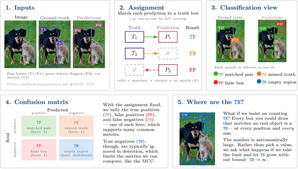
More specifically, to score an object detector, we are given a set of images, each with a set of ground truth boxes and a set of predicted boxes. We have an assignment algorithm that determines if a predicted box should be matched against a truth box. The details of how to do that can vary depending on your use case, but for the purpose of this article, we can abstract that step away. It’s not what I want to discuss here.

Once you have the assignment between truth and predictions, the problem simplifies dramatically. Each match or failure to match can be treated as a single example in a binary classification problem, which is much easier to understand.

A true box assigned to a predicted box is a true positive. A predicted box assigned to nothing is a false positive. A true box assigned to nothing is a false negative. But this leaves out one case: true negatives.

True Negatives in Object Detection

In object detection, a true negative is a case where there wasn’t an object of interest, and the algorithm correctly did not predict a box.

If you are using common object-detection metrics (e.g., precision, recall, false alarm rate, F1, etc.), this doesn’t matter. These measures don’t depend on the number of true negatives. All the existing tools were happy ignoring them.

But I wasn’t writing an existing tool. I was writing a software library (KWCoco) that I wanted to be principled and grounded, and I wanted to make the idea of casting object detection as binary classification explicit. Without a true negative count, I couldn’t compute all of the binary classification metrics I wanted to.

Specifically, at the time, I was interested in the Matthews Correlation Coefficient due to the work of David Powers. And if I couldn’t compute the MCC for my object detection problem, then I needed a good justification.

I could have said the MCC is undefined because the number of true negatives was zero. But that felt wrong. Think about it. If you have an object detection algorithm, you are correctly not placing boxes a lot! Think about every single 1×1 pixel box outside the truth objects. Every time you could have predicted one of those, but didn’t – that should be counted as a true negative. If you let the size of those boxes increase, then all the boxes of any size that don’t sufficiently overlap the truth should count too. Let’s take it further: what if we allow boxes with widths and heights greater than the image size? The number of true negatives becomes absurdly large.

So what if we take it to the extreme? What if we let the number of true negatives go to infinity? This is the question that led to the main result in the paper.

Taking True Negatives to the Limit

I expressed the limit of the MCC as TN goto in SymPy to check, and the equation simplified into something nice. I looked for existing work on the limit of the MCC and didn’t find anything. Perhaps I had found a niche result. I wrote a small blog post on it.

Later, a Reddit user observed that the formula was the geometric mean of precision and recall, which I later learned is called the Fowlkes-Mallows index (FM Index). So now, in addition to a formula, I had a geometric interpretation and a better label for what I was seeing. My original motivation for looking into this problem was to write software that cast detection as classification, and this justified omitting the MCC from detection metrics.

So I put the problem down for a while, but it remained in the back of my mind. Even though I had done the calculation in Sympy, I hadn’t done it by hand. I hadn’t really felt why it was true, and I wanted to.

It was late 2022 that I made time to work through it. I wrote up a proof in LaTeX, and then published it on arXiv. When I shared it with my co-workers, someone pointed out that I had made the proof more complicated than necessary. Their feedback made the proof simpler and clearer. Again, sharing my work had paid off: feedback from a colleague made the proof simpler and clearer. I updated the arXiv paper, and was fairly satisfied with where I had landed: a potentially novel result – at least nobody had framed it the way I had yet.

But there’s something about writing a proof on paper that’s bothered me. Ideally, you would write out each detail so that the steps are straightforward and anyone can verify it. But in practice, what often happens is that certain steps are left as exercises to the reader. Usually, they are obvious to the audience they were written for, but for others, they are often opaque.

In my case, the proof was fairly simple. I was confident it was correct, but I’m also human – and I happen to be the sort of human that enjoys going down epistemological rabbit holes. So, turning a skeptical lens inward, I asked myself: how can I prove to myself that I haven’t made a mistake? And how can I do this while minimizing the trust surface?

Towards verifying the proof

I wanted a system where the proof could be independently checked – a mechanized proof checker that I could trust. It turns out that these things exist: proof assistants. Particularly, I was interested in Lean4, a proof assistant that the mathematics community seemed to be gravitating towards. In addition to being fast and having a rich standard library, it also boasts a very small kernel to which all trust is delegated.

I now have the idea that I wanted to prove this in Lean. However, I quickly realized this was not going to be a simple task. What was nice was that for any Lean program I looked at, I could back-reference everything about it; even if the chain was long, it was explicit. Unfortunately, determining what I needed to prove my result was unclear

So I picked at the problem as I had time. I learned that I would need ideas from topology, such as Tendsto and atTop, and I worked on proving simpler results like lim_{x} 1/x = 0. And then, AI started to improve.

LLMs enter the picture

Early LLM attempts (GPT 4o) to help with the Lean proof were dead ends. But as the models improved (GPT 5.1), they became good enough to produce something close to a working formalization. After a few rounds of iteration, around November 2025, I had a proof that compiled. The statement was true, mechanically verified, and every step was explicit. There were no more questions.

Except, there were more questions. The proof compiled, but I still didn’t understand what the Lean code was doing. So I posted the proof and a challenge to do better on Zulip. The nerd snipe was successful. Two users helped me refine the proof further and gave me hints to better understand the Lean code.

So now I had a much cleaner formalization, one shaped not just by my own effort but also by feedback from others who understood Lean better than I did. And, to the best of my knowledge at the time, I had a novel result. But while thinking about how to include the formalization, I felt I needed to revisit the literature search. Previously, my Google searches had come back empty, but those were keyword-based searches. With LLMs, there is a new way to search for information semantically. I asked GPT 4o if my result was novel, and it told me, of course, that it was and that I’m actually the most insightful researcher in the world for finding it. But I thought I should try using the latest (GPT 5.2 at the time), and it pointed me at a paper: “Assessing species diagnostic value in large data sets: a comparison between phi coefficient and Ochiai index”. The paper was not about object detection or classifier evaluation; it was about measuring ecological association between species and vegetation, and the same mathematical relationship was noted there, but under different terminology. At a high level, the same math used to describe correlation between species populations also works for measuring the quality of machine learning algorithms.

Finding the Missing Result

The result wasn’t novel; it had been noticed before, but under a different name. The MCC is a form of the phi coefficient, and the FM-index is also known as the Ochiai index. I couldn’t help feeling disappointed, but now it was even more important to update the paper to include the missing reference. The LLM provided me with the pointer, but I needed to do the work to dig into it.

The 2008 paper was not available online, but I was able to contact the authors, who provided the full text. But when I looked at the paper, it stated the fact but didn’t provide the proof; instead, it cited a 1981 paper by Janson and Vegelius.

Again, the article was not available online, so I emailed the authors and received a copy. This time, I got the right paper. It was an interesting read. They use the phi coefficient (analogous to the MCC) as a way to measure correlation between the presence/absence of two species. They call out a “double zero” case in which an observation is made and both species are unobserved. This “double zero” is analogous to the true negative in object detection. The paper was motivated by finding measures that were insensitive to these “double zero” cases because, in their words, “a comparison between meadow flowers should not be influenced by the addition of localities from swamp and city areas.”

Finally, on page 4, after equation 20, I found the part I was interested in. I was eager to see the proof, but what I saw instead was:

As is easily seen, r_φ tends to r_O, when D tends to infinity.

Here, r_φ, r_O, and D are analogous to the MCC, FM-index, and number of true negatives.

…so, they left it as an exercise for the readers.

To be fair, the relationship is easy to see in the context of their other work. But this is exactly why I went down the formalization path to begin with. I don’t want to rely on results being easy to see. I want them to be explicit and (close to) impossible to refute.

So, the observation wasn’t new, but to the best of my knowledge, it is the first explicit proof, and almost certainly the first formal Lean4 proof.

Wrapping up

That’s the story of my recent update to my arXiv paper. For such a small observation, I’ve probably taken it far further than it needed to go, but that’s also what’s been fun about it.

I’m quite excited about the value AI added here. It helped me get the Lean proof over the finish line and made the connection to earlier work I had missed. But AI is only one part of the story.

Most of the value came from people communicating and sharing ideas. I think of the people who helped shape my understanding of this problem: the Redditor who pointed out the geometric mean, the colleague who simplified the handwritten proof, the Zulip users who shortened the Lean proof, the authors who sent me their work, and the countless other people who have contributed to our open knowledge and software ecosystems.

As I’m writing this story, I’m reminded how much value comes from our ability to communicate, share information, and collaborate. That’s what humans have done best for the past 10,000+ years. It’s my hope that AI will let us do more of that as we enter the next phase of the information age.

Glossary

Object detection: A computer vision task where an algorithm tries to find objects in images and draw boxes around them.

Groundtruth box: A box marking where an object really is in an image. These are usually created by human annotators and treated as the reference answer.

Predicted box: A box produced by an object detector. The detector is claiming that an object appears at that location.

Assignment algorithm: A method for matching predicted boxes to ground truth boxes. Once predictions are matched to truth, each prediction can be counted as correct, incorrect, or missed.

True positive (TP): A real object that the detector correctly found.

False positive (FP): A predicted object that does not match a real object.

False negative (FN): A real object that the detector missed.

True negative (TN): A case where there was no object and the detector correctly did not predict one. In object detection, this is tricky because there are many possible places where an object could have been predicted but was not.

Precision: Of the objects the detector predicted, the fraction that were correct. Informally: when the detector says “yes,” how often is it right?

Recall: Of the real objects present, the fraction that the detector found. Informally: how many of the real objects did it catch?

Matthews correlation coefficient (MCC): A balanced classification score computed from true positives, false positives, false negatives, and true negatives. It is also closely related to the phi coefficient.

Phi coefficient: A correlation coefficient for two binary variables. In the setting of a binary classification confusion matrix, it is equivalent to the MCC.

Fowlkes-Mallows index (FM index): The geometric mean of precision and recall.

Ochiai index: Another name for the same quantity as the Fowlkes-Mallows index, used in some ecological and similarity-measure contexts.

Proof assistant: Software for writing mathematical proofs in a form that a computer can check. In this article, Lean4 is the proof assistant used to verify the result.

Trust surface: The amount of reasoning, software, or human judgment that must be trusted for a result to be accepted. A smaller trust surface means fewer places where an unchecked mistake could hide.