Post-processing Smoothed-Particle Hydrodynamics (SPH) using ParaView

Following Kitware’s participation in the PARTICLES25 conference last October, including the presentation of a survey paper, this article provides an overview of current approaches for post-processing SPH data in ParaView.

Smoothed Particles Hydrodynamics, or SPH for short, is a mesh-free fluid simulation method used in a variety of fields, including hydrodynamics and astrophysics. SPH uses particles to represent mass: each particle has a position, a velocity, and discretizes continuous fields such as pressure in space using kernel functions around their position. Many physics solvers using SPH, such as DualSPHysics or OpenRadioss, can run in parallel on supercomputers, simulating billions of particles at once. This creates a challenge for visualization, as direct rendering of a large number of particles as points or spheres does not always give scientifically interesting results.

While a previous 2-part blog post covers in detail SPH interpolation techniques that can be used in ParaView, this post compares different SPH post-processing methods that you can use to explore your own data. Let’s dive in!

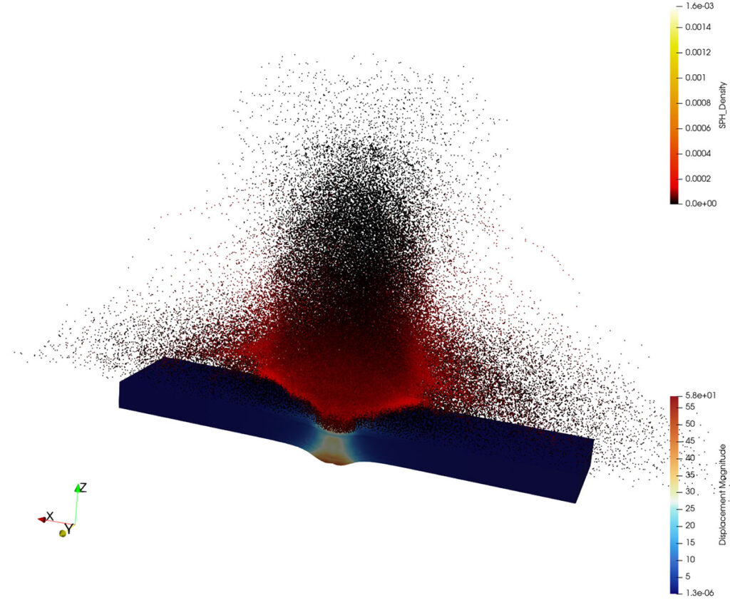
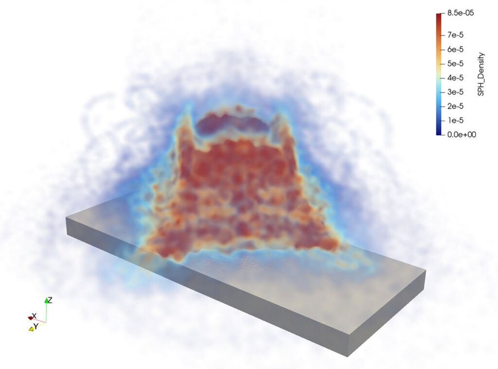
Figure 1: Visualization of a charge exploding on a concrete slab simulated by OpenRadioss

Direct Point Rendering Techniques

A first idea for a straightforward visualization of SPH points would be to draw them as color-mapped points, but even for smaller datasets, the result does not help much in understanding the particles’ organization and dynamics. Here is an example 3D rendering of a close-in explosion on a Concrete slab, simulated using OpenRadioss by Altair/Siemens:

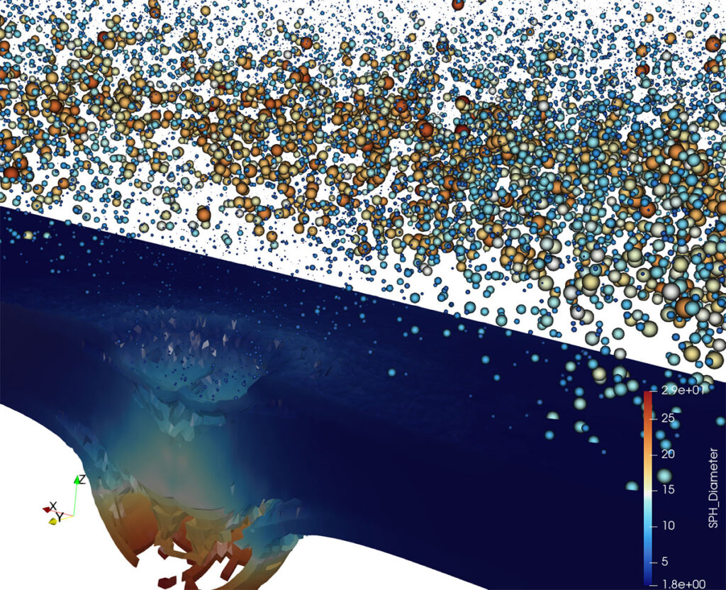
To reduce the visual noise caused by the large number of points, we can subsample points and try to keep the most relevant ones. A possible approach is to derive a histogram from the points being sampled, and select with a higher probability points that fall into bins where the fewest other points are. When sampling SPH particles based on pressure values using this histogram method, we retain extreme and rare values while discarding many particles in uniform regions. ParaView (since 6.0) provides a “VTKm Histogram Sampling” filter for this purpose. The output of this filter may be visualized directly using color-mapped spheres using the “Point Gaussian” representation in ParaView.

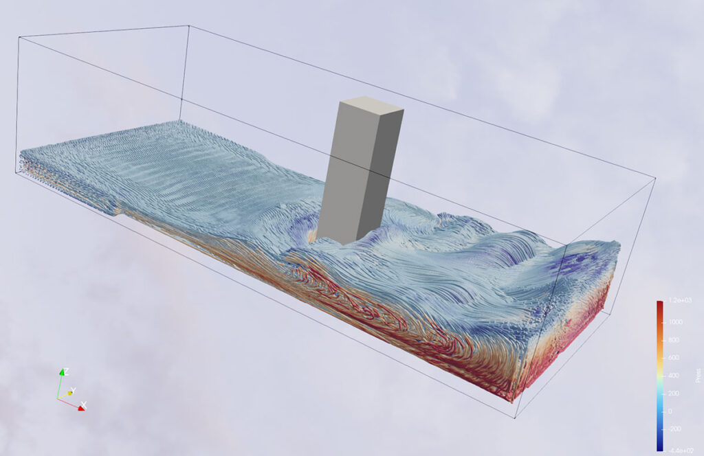
So far, we have only explored static visualization tools that do not account for time. Both fluid and shock simulations are to be analyzed as dynamic events. For that, ParaView provides a “Temporal Particles To Pathlines” filter that uses particle identifiers from the simulation to track points over a time window and draw the trail associated with their changing positions. This filter enables one to show the result of multiple time steps in a single picture, which is better suited for publication in a paper than a video.

For this example, we will use the DualSPHysics fluid solver, specifically, a Dam break case. DualSPHysics provides unique identifiers for SPH points, so we can track points’ positions over time and follow their trajectory. Figure 4 represents the SPH fluid simulation as particle pathlines over 50 time steps, randomly decimated, and colored using particle velocity magnitude. This representation shows how a given particle changes position and velocity over a time window. We are also using realistic path tracing rendering, providing shadows that enhance 3D perception and contrast.

SPH Grid Interpolation

As we demonstrated in the previous section, direct point rendering methods can be used to get a first look at the data, but fall short when scaling to millions of points. Methods involving point decimation lose crucial information about density and overlook SPH particle kernel functions. About 10 years ago, ParaView introduced interpolation filters for SPH, which integrate SPH kernels over a line, a 2D plane, or a volume.

Once points are interpolated into a regular grid, we can apply more classic scientific visualization algorithms, such as volume rendering, represented in Figure 5. We use a custom color and opacity transfer function to display the density in 3D space.

For the fluid simulation, we run an iso-contour algorithm to highlight the waterfront (Figure 7). The contour creates a surface at a given density iso-value, and colors it using the velocity value.

Figure 7. Pressure Isocontour on the fluid simulation, showing the waterfront, colored by the particle velocity field.

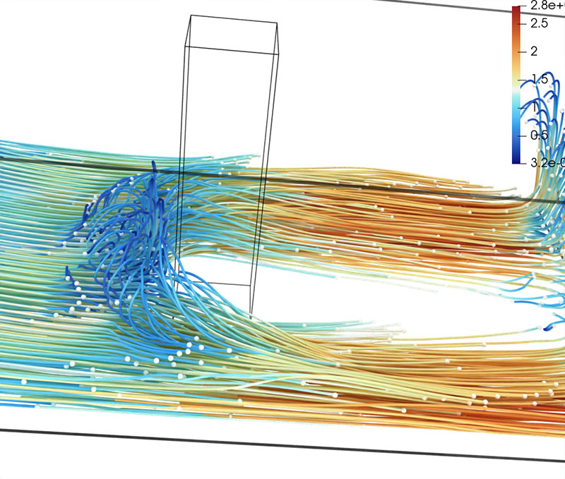
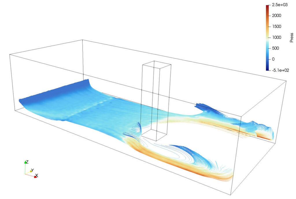
One last common visualization technique for CFD simulations is the use of streamlines, which show current lines of the vector velocity field. Once again, starting from the SPH particles interpolated over a volume, we set a starting line and trace current lines through the regular grid, preserving the velocity vector field for each particle (figure 9). This reveals the direction of travel of a fluid element at a given point in time.

Conclusion

This blog post highlights the characteristics of SPH simulation post-processing and visualization using ParaView. ParaView offers several filters to extract meaningful information, like the SPH Interpolators. Using real-world use cases simulated with DualSPHysics and OpenRadioss, we successfully explored the capabilities for retrieving relevant insights from SPH simulations.

We hope this blog post will stimulate discussion within the ParaView community about the challenges of post-processing modern SPH simulations! For any questions about this topic, do not hesitate to contact our team.